Building a Variational Autoencoder from Scratch: A Hands-on Guide with PyTorch + PIL

Why Variational Autoencoders Are Worth Learning Deeply

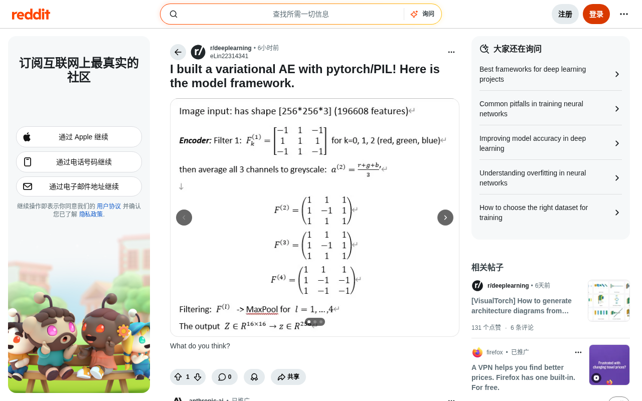
Recently, a developer shared their complete experience of building a Variational Autoencoder (VAE) from scratch using PyTorch and PIL in the Reddit community. Though concise, this post touches on a classic and fundamental core topic in the field of deep generative models.

Since VAEs were introduced by Kingma and Welling in 2013, they have remained an unavoidable cornerstone for understanding modern generative AI (diffusion models, GANs, etc.). Implementing a VAE by hand is not just an exercise in PyTorch operations—it's the most direct way to truly grasp how probabilistic generative models actually work.

reddit source: I built a variational AE with pytorch/PIL

What Is a Variational Autoencoder

The Historical Starting Point of VAE

In 2013, Diederik P. Kingma and Max Welling formally introduced the VAE framework in their paper Auto-Encoding Variational Bayes. The context of its introduction was the deep learning community's urgent need for generative models—at that time, GANs had not yet been born (GANs were proposed by Goodfellow in 2014), while traditional probabilistic graphical models such as Boltzmann machines were difficult to train and poorly scalable. VAE combined Variational Inference with deep neural networks, achieving for the first time a scalable probabilistic generative model on high-dimensional data, and pioneering a new paradigm for deep generative models.

Worth understanding in depth is the mathematical foundation of VAE—variational inference. Variational inference is a core method in Bayesian statistics for approximating complex posterior distributions. When exact computation of the posterior distribution p(z|x) is computationally infeasible, variational inference introduces a parameterized approximate distribution q(z|x), turning the inference problem into an optimization problem—namely, minimizing the KL divergence between q and the true posterior. VAE combines this statistical method with deep neural networks, using a neural network to parameterize q(z|x), thereby achieving Amortized Inference: each new data point does not require running a separate optimization process, but instead directly obtains the approximate posterior parameters through the encoder's forward pass. This makes it possible to train VAEs on large-scale datasets. It was precisely this innovation that quickly made VAE a foundational tool in generative AI research, and it directly influenced the architectural design of subsequent diffusion models.

Starting with the Ordinary Autoencoder

To understand VAE, we must first start with the Autoencoder. A traditional autoencoder consists of an Encoder and a Decoder: the encoder compresses input data into a low-dimensional latent representation, while the decoder reconstructs the original data from this latent representation.

The problem is that the latent space learned by an ordinary autoencoder tends to be discontinuous and irregular—you can't randomly sample from it to generate meaningful new data. This is precisely the core contradiction that VAE aims to solve.

The Key Innovation of VAE

The core breakthrough of the Variational Autoencoder lies in this: it encodes the input as a probability distribution rather than a fixed point. Typically a Gaussian distribution is used, described by a mean (μ) and a variance (σ). This makes the latent space continuous and smooth, allowing free sampling and thus the generation of entirely new data.

It is precisely this design that makes VAE a true generative model—by sampling in the latent space and decoding, it can produce new images that don't exist in the training set.

Key Technical Points of Implementing VAE in PyTorch

Three Core Components

Encoder Network: Maps the input image to the distribution parameters in the latent space. The final layer of the encoder outputs two sets of values, corresponding to the mean μ and the log variance log(σ²). Outputting the log variance rather than the variance itself ensures numerical stability while guaranteeing the variance is always positive.

Reparameterization Trick: This is the most ingenious design in VAE implementation. Sampling directly from a distribution would block the backpropagation of gradients, and the reparameterization trick offers an elegant solution:

z = μ + σ × ε, where ε is sampled from a standard normal distribution

The randomness is isolated into ε, allowing the gradients of μ and σ to flow normally, so the model can be trained end-to-end.

From a mathematical standpoint, if you sample directly from a distribution within the computational graph, the sampling operation itself is non-differentiable, and backpropagation breaks at this point. By decomposing the sampling into the formula above, the randomness is externalized as a noise input independent of the parameters, making μ and σ variables on a deterministic computation path, so gradients can flow back to the encoder normally via the chain rule.

The engineering value of this trick goes far beyond VAE itself. The reparameterization trick essentially solves the general problem of "backpropagating through random nodes" in deep learning: in reinforcement learning, continuous action space sampling in policy gradient methods (such as PPO, SAC) relies on the same idea; in diffusion models, the noise injection at each step of the denoising process uses a similar random variable parameterization; and in variational recurrent networks (VRNN) and stochastic residual networks, it is likewise a core building block. Mastering the reparameterization trick means acquiring a general tool for understanding how randomness is handled in many modern deep learning architectures—one of the few designs in the deep learning toolbox that combines both theoretical elegance and engineering practicality.

Decoder Network: Receives the latent vector z, maps it back to the original data space, and reconstructs the image output.

Loss Function: Both Parts Are Indispensable

The VAE loss function consists of two terms, and the balance between them directly determines the model's final performance:

Reconstruction Loss: Measures the difference between the reconstructed image and the original input, commonly using Mean Squared Error (MSE) or Binary Cross Entropy (BCE).
KL Divergence: Measures the distance between the latent distribution output by the encoder and the standard normal distribution. It acts as regularization, constraining the structure of the latent space to avoid "collapse" or "over-dispersion."

KL Divergence (Kullback-Leibler Divergence) is an asymmetric measure in information theory of the difference between two probability distributions. In VAE, the KL term constrains the distribution q(z|x) output by the encoder to be as close as possible to the standard normal prior p(z)=N(0,I). Its information-theoretic meaning is: how many extra bits the encoder needs to describe the deviation of the data distribution relative to the prior. When the KL weight is too small, the model ignores regularization and the latent space fragments (i.e., the "posterior collapse" problem, where each data point is mapped to nearly non-overlapping latent regions, making smooth interpolation impossible); when the weight is too large, the encoder is forced to compress all data into similar distributions, significantly degrading reconstruction quality. This trade-off was systematically studied in subsequent work, β-VAE (Higgins et al., 2017): by setting the KL term coefficient β to a value greater than 1, the model is forced to learn more disentangled latent representations, meaning different dimensions of the latent space correspond to different independent semantic factors of the data (such as color, shape, and pose in an image being controlled by independent dimensions). The emergence of β-VAE expanded VAE from a purely generative tool into an important framework for interpretable representation learning, with wide applications in fields requiring interpretable features such as medical image analysis and 3D scene understanding.

Tuning the weights of these two terms is the aspect of VAE parameter tuning that requires the most repeated refinement.

Processing Image Data with PIL

This developer chose PIL (Python Imaging Library) to handle image data processing—a very common pairing in computer vision projects. It's worth mentioning that the original PIL project is no longer maintained; modern Python projects actually use its active fork, Pillow (which is backward-compatible with the PIL interface). In deep learning vision pipelines, Pillow typically serves as the data entry point: reading formats like JPEG/PNG, performing resize/crop/color space conversion, and finally converting to tensors via torchvision.transforms or by manually calling numpy/torch.from_numpy. Compared with OpenCV, Pillow's API is more Pythonic and integrates more naturally with the torchvision ecosystem; compared with directly using torchvision's built-in datasets, manually processing custom datasets with Pillow gives developers more complete control over the data pipeline.

PIL handles preprocessing tasks such as image loading, resizing, and format conversion, then converts to PyTorch tensors to feed into the model. PIL handles image I/O, PyTorch handles model computation—a clear division of labor with well-defined responsibilities, and a standard practice pattern in many vision projects.

The True Value of Building from Scratch

Hands-on Work Builds Better Understanding Than Calling APIs

In today's era dominated by large models and packaged frameworks, why is it still worth writing a VAE from scratch?

The answer is the difference in depth of understanding. When you personally debug the reparameterization logic, balance the ratio of the two loss terms, and visualize the latent space distribution, your understanding of generative models will far exceed simply calling an interface.

More importantly, today's hottest diffusion models (such as Stable Diffusion) contain a VAE as a core module internally. The Latent Diffusion Model (LDM) is the theoretical foundation of Stable Diffusion, proposed by Rombach et al. in 2022. Its core idea is to move the diffusion process from pixel space to the VAE-encoded latent space, compressing the computational load by tens of times. Specifically, the VAE encoder compresses a 512×512 RGB image into a 64×64×4 latent tensor, the diffusion model performs denoising iterations in this low-dimensional space, and finally the VAE decoder restores it to a high-resolution image.

This architectural choice makes the quality of the VAE a critical bottleneck for the entire generation pipeline. The upper limit of Stable Diffusion's image quality is largely determined by the reconstruction fidelity of its built-in VAE—the detail information lost during VAE encoding cannot be recovered by the diffusion model out of thin air. This also explains why the community continuously attempts to replace or fine-tune the VAE component to improve output quality: from SD 1.x to SDXL, the official VAE has undergone multiple iterative upgrades in precision and color fidelity; third-party communities have also contributed specialized VAE variants optimized for specific styles (such as anime and portraits). For engineers who want to deploy or fine-tune diffusion models in production environments, the ability to independently evaluate and replace VAE components has become an indispensable technical reserve. Mastering VAE principles is a prerequisite for truly understanding cutting-edge generative AI architectures.

The Virtuous Feedback Loop of the Open Source Community

This developer proactively posted to showcase the framework and solicit community feedback, embodying the most valuable form of interaction in a technical community. Sharing not only helps oneself obtain suggestions for improvement, but also leaves a reference case for other learners.

Summary

Building a Variational Autoencoder from scratch is one of the most solid entry paths into the field of generative AI. PyTorch provides flexible model-building capabilities, PIL handles image preprocessing, and together they can walk through the complete chain from data to model.

VAE theory has sufficient depth—probabilistic modeling, variational inference, latent space constraints; the practice also has sufficient visibility—loss curves, reconstruction effects, latent space visualization. For learners who want to truly understand generative AI, this is a starting point worth spending time to master thoroughly.