Building a Neural Network from Scratch with NumPy: A Hands-On Deep Dive into Backpropagation
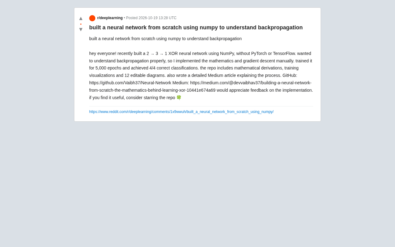
Reddit user builds a 2→3→1 XOR neural network from scratch with NumPy, fully covering forward propagation, backpropagation, and gradient descent, reaching 4/4 accuracy after 5,000 rounds.
A Reddit user built a 2→3→1 XOR neural network from scratch with NumPy, manually implementing forward propagation, backpropagation, and batch gradient descent to reach 4/4 classification accuracy after 5,000 training rounds. The project is open-sourced on GitHub with full mathematical derivations, loss curves, decision boundary visualizations, and 12 editable diagrams. The community notes that hand-written implementations deepen understanding of gradient flow and debugging, but are best suited for learning; real projects should still use frameworks like PyTorch.
Why Build a Neural Network from Scratch?
In an era dominated by PyTorch and TensorFlow, calling model.fit() has become almost reflexive. But one Reddit user (u/Vaibh37) took the opposite approach, building a 2→3→1 XOR neural network from scratch with NumPy — implementing forward propagation, backpropagation, and gradient descent in full, reaching 4/4 classification accuracy after 5,000 training rounds. The project is open-sourced on GitHub, complete with detailed mathematical derivations and 12 editable diagrams.
This isn't reinventing the wheel — it's a learning experiment in "deconstructing the black box." As the author put it: "I wanted to truly understand backpropagation, so I implemented the math and gradient descent by hand." For anyone looking to solidify their deep learning foundations, this kind of exercise is far more valuable than just calling libraries.
Project Breakdown: From Math to Code
Network Architecture: Minimal but Complete
The network uses 2 input nodes, 3 hidden nodes, and 1 output node, with Sigmoid activation and mean squared error (MSE) loss. The four XOR samples ((0,0)→0, (0,1)→1, (1,0)→1, (1,1)→0) are not linearly separable, requiring a hidden layer to learn the nonlinear relationship. Choosing such a small network ensures every step of the computation can be verified by hand, avoiding dimensional complexity that would obscure understanding.
Mathematical Derivation of Backpropagation
The author provides complete mathematical derivations in the GitHub repository, covering the layer-by-layer application of the chain rule: from the gradient of the loss with respect to the output layer to the weight updates in the hidden layer. Key formulas include:
- Output layer error term: δ_out = (a_out - y) * σ'(z_out)
- Hidden layer error term: δ_hidden = (W_out^T · δ_out) * σ'(z_hidden)
- Weight gradient: ∂L/∂W = δ · a_prev^T
These formulas are implemented line by line in code, without any automatic differentiation. The author also visualized the computation graph through 12 editable diagrams (likely using draw.io or similar tools) to help readers track gradient flow.
Sigmoid activation function and its derivative: The Sigmoid function is defined as σ(z) = 1 / (1 + e^{-z}), and its derivative takes the elegant form σ'(z) = σ(z)(1 - σ(z)). This property makes it very convenient to compute the gradient of the activation function during backpropagation — you only need the activation values saved during forward propagation. In the XOR network, both the hidden and output layers use Sigmoid, so σ'(z) in the error term calculation can be directly replaced by a(1 - a).
Mean squared error (MSE) loss function: MSE is defined as L = (1/n) * Σ(a_out - y)^2, where n is the number of samples. For a single sample, the loss is (a_out - y)^2, and its gradient with respect to the output layer is 2(a_out - y) * σ'(z_out). The formula δ_out = (a_out - y) * σ'(z_out) in the article omits the constant factor 2, which in practice doesn't affect the direction of gradient descent — it's equivalent to a scaling of the learning rate. With MSE and Sigmoid, the output layer gradient includes the σ'(z_out) term, which shrinks as outputs approach 0 or 1 — a phenomenon worth noting in early network training.
Training and Visualization
The training process uses batch gradient descent with a manually tuned learning rate over 5,000 iterations. The repository includes training loss curves and decision boundary visualizations, intuitively showing how the network gradually partitions the XOR space. The final 4/4 classification result, though simple, validates the correctness of the implementation.
Batch Gradient Descent: Batch gradient descent computes the loss gradient using all training samples in each iteration, then updates the weights once. For the 4 XOR samples, this means each update is based on the average gradient across all samples — stable in direction but with computational cost growing linearly with sample count. In contrast, stochastic gradient descent (SGD) and mini-batch gradient descent are more commonly used in deep learning. With so few samples in this project, batch gradient descent is entirely feasible and clearly demonstrates the deterministic trajectory of gradient descent.
Decision boundary visualization: The decision boundary is the contour where the classifier output equals 0.5, appearing as a curve in the 2D input space. For the XOR problem, since the data is not linearly separable, the decision boundary must be nonlinear. By plotting the decision boundary, you can intuitively see how the hidden layer warps the input space so that the output layer can partition it linearly. Visualization typically involves densely sampling a grid in the input space, running forward propagation to get output values, and then using Matplotlib's contourf function to plot them.
Multi-Source Perspectives: The Value and Limitations of Hand-Written Implementations
This project sparked discussion on Reddit's r/MachineLearning. According to post comments and the author's description in a Medium article, the main benefits of hand-written implementation are:
- Deeper understanding of gradient flow: After deriving the chain rule by hand, you have a much clearer picture of what's happening under the hood when using PyTorch's
autograd. - Improved debugging skills: When a model doesn't converge, you can quickly identify whether it's vanishing gradients, too large a learning rate, or an initialization problem.
- Educational value: Clear mathematical derivations and visualizations make it suitable as an introductory tutorial.
But some comments also pointed out limitations: NumPy implementations are only suitable for teaching; in real projects, manually computing gradients is inefficient and error-prone, especially with complex structures like convolutions and attention. Moreover, the XOR problem is too simple to demonstrate challenges like vanishing/exploding gradients in deep networks.
The author responded to these points in the Medium article, acknowledging that the project's purpose is "understanding" rather than "production," and recommending that beginners transition to frameworks after mastering the fundamentals — but not skip the hand-written stage.
How to Reproduce and Extend Your Learning
If you want to reproduce this project, follow these steps:
- Clone the GitHub repository (Vaibh37/Neural-Network).
- Install NumPy and Matplotlib.
- Run the training script and observe the loss curve and classification results.
- Modify the network architecture (e.g., add more hidden nodes) or activation function (e.g., ReLU) and compare results.
Suggestions for further learning:
- Try implementing multi-class classification (e.g., the Iris dataset) using the same approach, changing the output layer to Softmax.
- Add a regularization term (L2) and observe its effect on the weights.
- Use numerical gradient checking to verify the correctness of your backpropagation implementation.
These exercises will further solidify your understanding of backpropagation.
Numerical gradient checking: Numerical gradient checking is a method to verify whether analytically computed gradients (from backpropagation) are correct. The principle is to approximate derivatives using finite differences: for each parameter θ, compute [L(θ+ε) - L(θ-ε)] / (2ε), where ε is a very small number (e.g., 1e-4). Compare the numerical gradient with the analytical gradient from backpropagation; if the relative error is less than 1e-7, the implementation is generally considered correct. In complex networks, gradient checking is the gold standard for debugging backpropagation, but it's computationally expensive and used only for verification, not training.
Softmax and multi-class classification: The Softmax function converts the raw scores of multiple output neurons into a probability distribution: softmax(z_i) = e^{z_i} / Σ_j e^{z_j}. Combined with cross-entropy loss, Softmax output layers are commonly used for multi-class tasks. Unlike Sigmoid for binary classification, Softmax ensures that all class probabilities sum to 1, and its gradient takes a clean form (δ_out = a_out - y). To extend the XOR network to multi-class classification, change the output layer to multiple nodes with Softmax and switch the loss function to cross-entropy.
Conclusion: Foundations Determine the Ceiling
In an age of increasingly encapsulated AI tools, occasionally returning to low-level hand-written code is precious training for technical intuition. This NumPy neural network project is small, yet it completely covers the core mathematics of deep learning. As the author said at the end of the post: "If this is helpful to you, consider giving the repo a star." — Perhaps that's the best footnote to the open-source learning spirit.
One-line Summary
A Reddit user built a 2→3→1 XOR neural network from scratch with NumPy, fully covering forward propagation, backpropagation, and gradient descent, achieving 4/4 classification accuracy after 5,000 training rounds.
Paragraph Summary
A Reddit user built a 2→3→1 XOR neural network from scratch with NumPy, manually implementing forward propagation, backpropagation, and batch gradient descent, reaching 4/4 classification accuracy after 5,000 training rounds. The project is open-sourced on GitHub with complete mathematical derivations, training loss curves, decision boundary visualizations, and 12 editable diagrams. The author's goal was to truly understand the mathematics of backpropagation, not to reinvent the wheel. Community discussion notes that hand-written implementations deepen understanding of gradient flow, improve debugging skills, and have educational value — but also points out they're only suitable for teaching; real projects should still use frameworks like PyTorch. The author recommends that beginners transition to frameworks after mastering the fundamentals, but not skip the hand-written stage.
Related articles

RAG Getting Started in Practice: From Principles to Building an Enterprise Knowledge Base
Bilibili RAG course highlights: from retrieval-augmented generation principles, document chunking and vectorization, to five accuracy factors and enterprise knowledge base boundaries, with fine-tuning vs RAG selection advice.

AI Model Selection Guide: DeepSeek vs. Qwen3 in Practice
How should AI developers choose models? Based on a Bilibili tutorial, this article breaks down the Function Calling differences between DeepSeek V3 and R1, Qwen3's programmatic thinking mode switching and agent capabilities, and outlines a multi-model learning path and practical selection logic.

Anchoring, Loss Aversion, and Nudges: 5 Psychological Tactics Retailers Use to Make You Spend
Behavioral economics reveals how retailers use anchoring, framing, loss aversion, and nudge theory to manipulate your spending decisions. This article breaks down 5 common psychological tactics and offers counterstrategies like slowing down decisions and setting your own anchors to see through the pricing design behind discounts.