Confusion Matrix Explained: Precision, Recall, and F1 Score Formulas with Practical Applications

Introduction

Regression models measure the deviation between predicted and actual values, while classification models measure how many predictions are correct. So how do you scientifically evaluate a classifier's performance? This is where the Confusion Matrix comes in, along with its derived metrics: Accuracy, Precision, Recall, and F1 Score.

This article starts with the basic concepts of the confusion matrix, progressively breaks down each metric's calculation method, and combines three real-world scenarios—spam detection, financial fraud prevention, and cancer screening—to help you understand which metric to focus on under different business contexts.

Confusion Matrix: The Foundation of Classification Evaluation

The Four Core Concepts: TP, TN, FP, FN

A confusion matrix is an M×M table (2×2 for binary classification), where rows represent the actual class of samples and columns represent the model's predicted class. In binary classification, there are four key terms:

• TP (True Positive): The actual class is positive, and the model also predicts positive. For example, if 90 out of 100 cats are correctly identified as cats, then TP=90.
• TN (True Negative): The actual class is negative, and the model also predicts negative. For example, 100 dogs are correctly identified as "not cats."
• FP (False Positive / False Alarm): The actual class is negative, but the model incorrectly predicts positive.
• FN (False Negative / Miss): The actual class is positive, but the model incorrectly predicts negative.

A simple memory trick: The first letter T/F indicates whether the prediction is correct, and the second letter P/N indicates the model's predicted result. True Positive means "prediction correct + predicted as positive," and False Positive means "prediction wrong + predicted as positive."

Historical Origins and Multi-class Extension

The concept of the confusion matrix can be traced back to Karl Pearson's research on classification errors in statistics in 1904, and was later systematized in Signal Detection Theory. During World War II, radar operators needed to distinguish enemy aircraft signals from noise interference, and the TP/FP/TN/FN framework was formally established in this military context—"true positives" corresponded to correctly identified enemy aircraft, and "false positives" corresponded to false alarms where noise was mistaken for enemy aircraft.

For multi-class problems (such as handwritten digit recognition with 10 classes from 0-9), the confusion matrix expands into an M×M square matrix. Each element on the diagonal represents the number of correctly classified samples for a given class, while off-diagonal elements reveal specific confusion patterns—for example, the digit "3" is often misclassified as "8," and "1" is easily confused with "7." This fine-grained error analysis is extremely valuable for model improvement, allowing developers to specifically add training samples for easily confused classes or adjust feature engineering strategies.

What Does an Ideal Confusion Matrix Look Like?

In a good classifier's confusion matrix, the diagonal elements (TP and TN) should be as large as possible, while the off-diagonal elements (FP and FN) should be as close to zero as possible. The more correct predictions and fewer errors, the better the model.

Core Evaluation Metrics and Formulas

Accuracy: Most Intuitive but Not Always Reliable

The formula for accuracy is:

$$Accuracy = \frac{TP + TN}{P + N}$$

The meaning is straightforward: the proportion of correctly predicted samples out of total samples.

Using cancer detection as an example, suppose there are 10,000 cases where correct detections and correct exclusions add up to 9,989, the accuracy would be 9989/10000 = 99.89%.

However, accuracy has a fatal flaw: it can be misleading when samples are severely imbalanced. For example, in cancer screening where positive samples are extremely rare, a model that predicts everyone as healthy can still achieve over 99% accuracy, yet such a model has no practical value.

Class Imbalance: The Root Cause of Accuracy Failure

Class Imbalance is one of the most common practical challenges in machine learning. In real datasets, positive-to-negative sample ratios of 1:100 or even 1:10000 are not uncommon. For example, in credit card fraud detection, fraudulent transactions typically account for less than 0.1% of total transactions; in network intrusion detection, malicious traffic may constitute only one ten-thousandth of all traffic.

To address this, beyond selecting appropriate evaluation metrics, the industry has developed multiple strategies: oversampling techniques (such as SMOTE, which generates synthetic samples by interpolating between minority class samples), undersampling techniques (randomly reducing majority class samples), cost-sensitive learning (assigning different penalty weights to different types of errors), and ensemble methods like EasyEnsemble and BalanceCascade. Understanding why class imbalance causes Accuracy to fail is a key prerequisite for mastering classification evaluation metrics.

Error Rate

Error rate is complementary to accuracy:

$$Error\ Rate = 1 - Accuracy = \frac{FP + FN}{P + N}$$

This is the proportion of incorrectly predicted samples out of total samples.

Precision: The Key Metric for Measuring False Alarms

Precision answers the question: Of all samples predicted as positive, how many are actually positive?

$$Precision = \frac{TP}{TP + FP}$$

For example: if a model predicts 10 samples as positive, with 9 actually being positive and 1 being a false alarm, then precision is 9/(9+1) = 90%. Higher precision means fewer false alarms from the model.

Recall: The Key Metric for Measuring Misses

Recall answers the question: Of all actual positive samples, how many were successfully identified by the model?

$$Recall = \frac{TP}{TP + FN}$$

Higher recall means fewer missed positives.

The Core Difference and Trade-off Between Precision and Recall

Precision and recall often have an inverse relationship. Raising the classification threshold makes the model more "conservative"—it only predicts positive when very confident—causing precision to rise but recall to fall. Lowering the threshold has the opposite effect: the model becomes more "aggressive," recall rises but precision drops.

Understanding this trade-off relationship is the prerequisite for choosing the correct evaluation metric.

Visualizing the Trade-off with PR Curves and ROC Curves

The trade-off between precision and recall can be visually demonstrated through PR Curves (Precision-Recall Curves) and ROC Curves (Receiver Operating Characteristic Curves). Most classification models don't output direct class labels but rather a probability of belonging to the positive class (e.g., logistic regression outputs a probability between 0 and 1). The classification threshold determines the probability above which a sample is classified as positive—the default is usually 0.5, but in practice it often needs to be adjusted based on the scenario.

The ROC curve uses FPR (False Positive Rate) as the x-axis and TPR (True Positive Rate, i.e., Recall) as the y-axis. The area under the curve, AUC (Area Under Curve), is a comprehensive evaluation metric unaffected by threshold selection—AUC=1 represents a perfect classifier, and AUC=0.5 is equivalent to random guessing. When classes are severely imbalanced, PR curves better reflect the model's true performance than ROC curves, because the FPR in ROC curves gets "diluted" by the large number of true negatives, making the model appear better than it actually performs.

F1 Score: The Harmonic Mean of Precision and Recall

The F1 score achieves a balance between precision and recall:

$$F1 = \frac{2 \times Precision \times Recall}{Precision + Recall}$$

The F1 score is only high when both precision and recall are relatively high. If either metric is extremely low, the F1 score will be significantly dragged down. It's particularly suitable for scenarios that need to balance both false alarms and misses.

Fβ Score: Flexibly Adjusting the Weight Between Precision and Recall

The F1 score is actually a special case of the Fβ score when β=1. The general formula for the Fβ score is:

$$F_\beta = \frac{(1+\beta^2) \times Precision \times Recall}{\beta^2 \times Precision + Recall}$$

When β>1, Recall carries more weight, suitable for scenarios where the cost of misses is high. When β<1, Precision carries more weight, suitable for scenarios where the cost of false alarms is high. For example, in financial fraud prevention, F2 score (β=2) can be used to emphasize recall more; in spam filtering, F0.5 score (β=0.5) can be used to emphasize precision more.

Additionally, in multi-class scenarios, F1 scores have two common aggregation methods: Macro-F1 (calculates F1 for each class separately then takes the arithmetic mean, treating all classes equally) and Micro-F1 (aggregates TP/FP/FN across all classes first then calculates a unified F1, dominated by classes with more samples). When class distributions are uneven, the difference between the two can be very significant, and choosing which aggregation method to use also depends on business requirements.

Practical Scenarios: Which Metric to Prioritize for Different Businesses

After understanding the formulas, the real challenge is: which metric should you prioritize in actual business scenarios? There's only one core criterion—between false alarms and misses, which one costs more.

Quantifying Business Costs with Decision Cost Matrices

In practice, choosing an evaluation metric is essentially conducting a cost-benefit analysis. A Decision Cost Matrix (Cost Matrix) associates each prediction outcome with specific economic or social costs. Taking financial fraud prevention as an example, a missed fraudulent transaction could cause losses of tens of thousands of dollars, while a false alarm merely costs the user an extra 30 seconds for identity verification. If the miss cost is $50,000 and the false alarm cost is $10, then the cost of a miss is 5,000 times that of a false alarm—this quantitatively explains why high Recall must be prioritized.

In industrial practice, data scientists typically work with business stakeholders to quantify these costs, then determine the optimal classification threshold and model selection strategy by minimizing expected total cost, rather than simply maximizing a single metric. This cost-based decision framework elevates model evaluation from "comparing technical metrics" to "optimizing business value."

Spam Detection: High Precision First

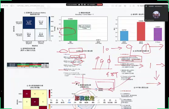
The principle of spam filtering is better to miss spam than to falsely flag legitimate emails.

Suppose there are 990 legitimate emails and 10 spam emails. Missing 1 spam email means the user sees one irrelevant message at most—limited impact. But if 1 legitimate email is incorrectly classified as spam and sent to the junk folder, the user might miss an important business email with much more serious consequences.

Therefore, spam detection requires high Precision to ensure that emails flagged as spam are actually spam.

Financial Fraud Prevention: High Recall First

Financial fraud prevention takes the opposite strategy: better to flag a thousand legitimate transactions than to let one fraud slip through.

Suppose out of 1,000 transactions, there are 100 fraudulent and 900 legitimate ones. Falsely flagging a few legitimate transactions as fraud at most requires users to do an extra identity verification—slightly degraded experience. But missing even one truly fraudulent transaction could cause enormous financial losses.

Therefore, financial fraud prevention requires high Recall to minimize the miss rate.

Cancer Screening: Better to Over-diagnose Than to Miss

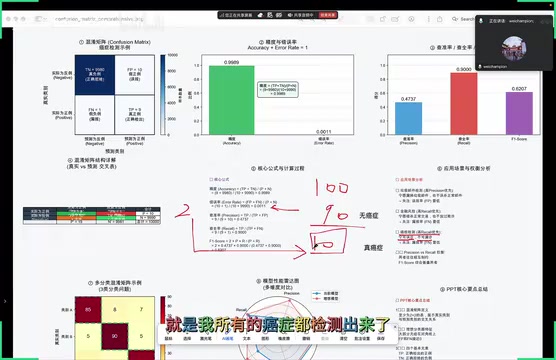
Cancer screening, like financial fraud prevention, is a typical scenario where high Recall takes priority.

Suppose out of 100 patients, 90 are healthy and 10 actually have cancer. Even if 2 healthy individuals from the 90 are "over-diagnosed" as suspected cases, they can be ruled out through further examinations. But if 4 out of 10 cancer patients are missed, these patients will miss their optimal treatment window with unimaginable consequences.

Metric Selection Quick Reference Table

Scenario	Priority Metric	Core Principle	Recommended Fβ Parameter
Spam Detection	Precision	Better to miss than to falsely flag	F0.5 (β=0.5)
Financial Fraud Prevention	Recall	Better to falsely flag than to miss	F2 (β=2)
Cancer Screening	Recall	Better to over-diagnose than to miss	F2 (β=2)
Balanced Scenarios	F1 Score	Balance both precision and recall	F1 (β=1)

A simple rule of thumb: For any scenario involving "money" or "lives," the cost of misses far exceeds the cost of false alarms, and high Recall must be prioritized.

Summary: How to Choose the Right Classification Evaluation Metric

The confusion matrix is the foundational tool for classification model evaluation, and its derived metrics—Accuracy, Precision, Recall, and F1 Score—each have different emphases:

• Accuracy is suitable for routine scenarios with balanced samples but can be misleading with class imbalance.
• Precision focuses on false alarms and is suitable for scenarios where false alarm costs are high, such as spam filtering.
• Recall focuses on misses and is suitable for scenarios where miss costs are high, such as financial fraud prevention and medical diagnosis.
• F1 Score balances precision and recall, suitable for scenarios where neither can be too poor.
• Fβ Score provides more flexible weight adjustment, allowing you to choose an appropriate β value based on the relative costs of false alarms and misses in your business.
• AUC-ROC and PR Curves evaluate the model's comprehensive performance across different thresholds from a global perspective, serving as important references during model selection.

No single metric is universal. Choosing the right evaluation metric is what enables you to make correct trade-offs during model tuning—and that is the core value of classification model evaluation.