Deep Dive into the Adam Optimizer: A Complete Guide to Adaptive Moment Estimation

Introduction

Adam (Adaptive Moment Estimation) is one of the most widely used optimizers in deep learning. It elegantly combines momentum with adaptive learning rates, making it suitable for virtually all computer vision tasks. This article breaks down the three core steps of the Adam optimizer from first principles, helping you truly understand why it achieves a balance between convergence speed and training stability.

Historical Background and Motivation Behind Adam

Adam was proposed by Diederik P. Kingma and Jimmy Ba in 2014 and published at ICLR 2015, in a paper titled Adam: A Method for Stochastic Optimization. Its creation stemmed from the deep learning community's long-standing exploration of two problems: how to make optimizers automatically adapt to gradient scale differences across parameters, and how to maintain stable convergence in noisy gradient environments.

Adam can be understood as an evolved version of AdaGrad and RMSProp — AdaGrad achieves adaptiveness by accumulating historical squared gradients, but causes the learning rate to monotonically decrease until updates cease; RMSProp replaces accumulation with exponential moving averages, solving the vanishing learning rate problem; Adam further introduces first-order moments (momentum) on top of this and adds a bias correction mechanism, enabling accurate moment estimates even in the early stages of training.

First Moment Estimation: Capturing Gradient Momentum

The first core component of Adam is the first moment estimation, which is essentially the computation of momentum.

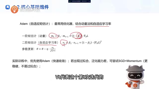
The formula for first moment estimation is:

$$m_t = \beta_1 \cdot m_{t-1} + (1 - \beta_1) \cdot g_t$$

Where:

• $m_t$ represents the first moment estimate at iteration $t$
• $g_t$ is the current gradient
• $\beta_1$ is the decay coefficient for the first moment (typically defaults to 0.9)

The Mathematical Essence of Exponential Moving Average

Both the first and second moment calculations in Adam are based on the Exponential Moving Average (EMA). EMA is a weighted averaging method where observations closer to the current time step receive higher weights, while older observations decay exponentially. Taking the first moment as an example, expanding the recursive formula reveals:

$$m_t = (1-\beta_1)\sum_{i=1}^{t}\beta_1^{t-i}g_i$$

This means the current moment estimate is a weighted sum of all historical gradients, with weights summing close to 1. The advantage of this design is that it only needs to store the moment estimate from the previous time step — minimal memory overhead — yet it implicitly "remembers" the entire training history. The larger the decay coefficient, the longer the effective window and the stronger the smoothing effect. This also explains why $\beta_2=0.999$ has a longer historical memory than $\beta_1=0.9$ — the second moment requires a more stable estimate of gradient variance.

The Role of Decay Coefficient β₁

$\beta_1$ controls how much historical momentum influences the current update:

• Large $\beta_1$ values (e.g., 0.99): $(1-\beta_1)$ is very small, the current gradient carries less weight, historical momentum has stronger inertia, and the update direction is smoother
• Small $\beta_1$ values (e.g., 0.5): $(1-\beta_1)$ is larger, the current gradient has more influence, and the response is more sensitive

The core value of first moment estimation lies in capturing the overall trend of gradients through exponential moving averages, preventing individual gradient noise from causing excessive disturbance to parameter updates. It's like a ball with mass rolling on the loss surface — it won't easily stop because of small local dips.

Second Moment Estimation: Achieving Adaptive Learning Rates

After obtaining momentum characteristics, Adam uses second moment estimation to achieve adaptive learning rate adjustment.

The formula for second moment estimation is:

$$v_t = \beta_2 \cdot v_{t-1} + (1 - \beta_2) \cdot g_t^2$$

Where:

• $v_t$ represents the second moment estimate at iteration $t$
• $g_t^2$ is the square of the current gradient
• $\beta_2$ is the decay coefficient for the second moment (typically defaults to 0.999)

Why Squared Gradients Are Needed

The second moment estimation tracks the exponential moving average of squared gradients, reflecting the fluctuation magnitude of gradients:

• When a parameter's gradient is consistently large and highly volatile, $v_t$ will be large, and the subsequent update step size will be reduced
• When a parameter's gradient is consistently small and stable, $v_t$ will be small, and the step size will be relatively increased

This is the essence of "adaptive