Deep Dive into vLLM's Scheduling Mechanism: The Complete CPU-to-GPU Mapping Pipeline
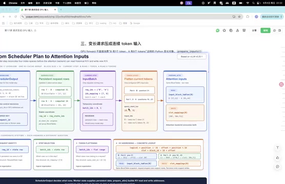
How vLLM maps CPU scheduling decisions to GPU physical memory through four index spaces.
This article provides a deep dive into vLLM's scheduling-to-execution pipeline, explaining how the inference engine converts CPU-side scheduler output into GPU-consumable input tensors. It covers persistent request state management, dual-index design, batch construction, token sequence flattening, and the multi-layer coordinate conversion chain that maps logical KV Cache blocks to physical GPU memory addresses.
The Core Challenge of vLLM's Schedule Conversion
As a high-performance LLM inference engine, vLLM's scheduler produces schedule output that is merely CPU-side control information — it cannot be directly consumed by the GPU. This article systematically explains how vLLM converts scheduling plans into GPU input tensors and how it precisely determines the physical write locations for KV Cache.
vLLM is an open-source LLM inference serving framework developed by UC Berkeley's Sky Computing Lab. Its core innovation is the PagedAttention mechanism, which borrows from operating system virtual memory management by dividing the KV Cache into fixed-size blocks for management, dramatically improving GPU memory utilization. In traditional inference frameworks, each request's KV Cache must occupy contiguous GPU memory, resulting in significant memory fragmentation. vLLM's paging approach enables non-contiguous KV Cache storage, boosting memory utilization from roughly 50% in conventional approaches to nearly 98%. This is precisely why a complex, multi-layered mapping exists between the control information produced by the scheduler and the physical addresses the GPU actually needs.
This conversion process involves multiple layers of coordinate mapping: from request IDs to global indices, from global state to batch indices, from discrete requests to contiguous token sequences, and finally to physical GPU memory addresses. Mastering these mappings is key to understanding vLLM's internal mechanics.
Worker Request State Management
Persistent Request Context Strategy
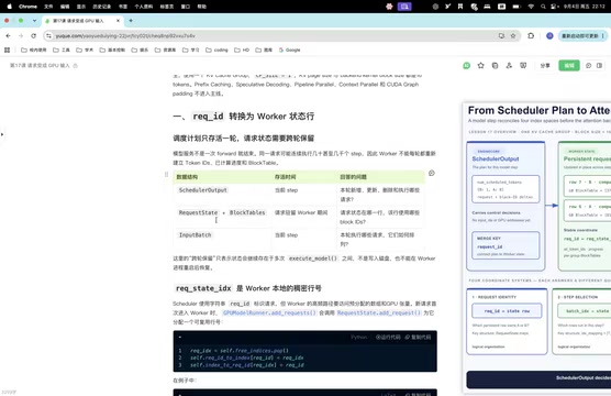
Model inference is a multi-step process — a single request requires multiple steps to complete. LLM inference consists of two phases: prefill and decode. The prefill phase processes all input tokens at once and generates the first output token, while the decode phase generates one new token per step. Due to the autoregressive nature of generation, each decode step must access the KV Cache from all preceding tokens. Therefore, the worker must persist request state and computation progress to avoid redundantly rebuilding context. The core data structures include:
- request_state: Tracks the computation progress of each request (e.g.,
completed_tokens), recording how many tokens have been processed so far and thus determining where the next computation step should resume. - block_table: Maintains the mapping from logical blocks to physical block IDs. Its design is analogous to an OS page table — logical blocks represent contiguous KV Cache space from the request's perspective, while physical block IDs correspond to the actual block locations allocated in GPU memory. This indirect mapping allows non-contiguous physical memory allocation, thereby eliminating memory fragmentation.
Schedule output is only valid for the current step; after execution, the scheduler generates a new output. The worker must update its persistent state accordingly to maintain continuity.
Design Logic Behind the Dual-Index System
The scheduler identifies requests using string request_ids, but the worker uses array indices (request_state_index) for better access performance. While string hash lookups have O(1) time complexity, their constant factor is relatively large. Array index access requires only a single memory offset calculation, and in high-frequency call scenarios, the performance difference is significant. When a new request arrives, an index is assigned; when a request completes, the index is recycled for reuse. This pooling strategy avoids the overhead of frequent memory allocation and deallocation.
Concrete example:
- Request B is assigned to row 7 (index=7): 31 tokens completed, physical block IDs are 37 and 12
- Request A is assigned to row 6 (index=6): 16 tokens completed, physical block IDs are 81 and 44
State management methods:
add_request(): Initializes state and block_table for a new requestupdate_request(): Appends newly allocated block IDs for an already registered request
Batch Construction and Sequence Flattening
Extracting the Execution Batch from Global State
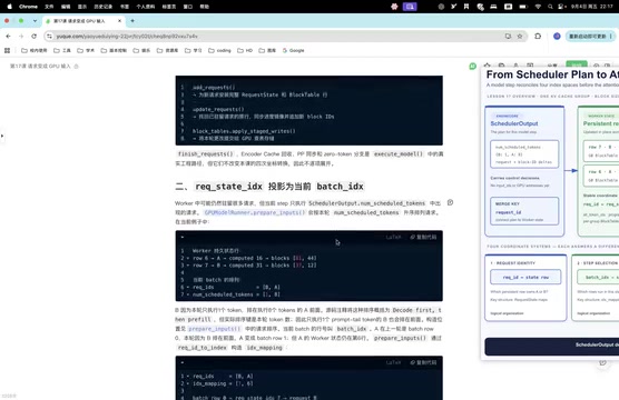
The schedule output specifies the current round's execution plan: Request B executes 1 token, Request A executes 8 tokens. The worker's execution flow:
- Extract the relevant requests from global state
- Sort by the number of tokens to execute in this round
- Assemble into a new batch
This introduces a new mapping relationship: Request B maps from global row 7 to batch row 2, and Request A maps from global row 6 to batch row 1. An index_mapping maintains this correspondence. This design allows the batch to be compactly arranged without wasting compute resources on empty rows in the global state table.
Contiguous Token Sequence Processing
GPUs cannot directly execute discrete token groupings. The GPU's SIMT (Single Instruction, Multiple Threads) architecture achieves peak efficiency when processing contiguous, regular data. Sending tokens from different requests to the GPU separately would incur substantial kernel launch overhead and GPU idle cycles. Therefore, "Request B's 1 token + Request A's 8 tokens" must be flattened into a contiguous sequence of 9 tokens to maximize GPU throughput. This sequence flattening technique, combined with fused kernels like FlashAttention, enables all requests' computations to be completed in a single GPU invocation.
After flattening, boundary information is preserved through the following arrays:
- query_start_loc: Records the starting position of each request. For example, [0, 1, 9] means token 0 belongs to Request B and tokens 1–8 belong to Request A. This array uses prefix-sum encoding — essentially a variant of the Compressed Sparse Row (CSR) format. The attention kernel uses it to distinguish request boundaries within a single contiguous computation, preventing cross-request attention leakage (i.e., ensuring Request A's tokens do not attend to Request B's KV Cache).
- position: Records each token's position within its original request. Request B's token in this round is at position 31; Request A's tokens are at positions 16–23. This information is critical for positional encoding mechanisms like RoPE (Rotary Position Embedding), ensuring each token receives the correct positional encoding consistent with its position in the original sequence.
- input_ids: Stores the actual token IDs, copied from the corresponding positions in the output's
token_ids.
These three arrays together enable reverse mapping from the contiguous sequence back to the original requests.
Precise Physical Address Mapping for KV Cache
Multi-Layer Coordinate Conversion Pipeline
Once the contiguous token sequence is obtained, the ultimate goal is to determine the read/write locations in GPU memory. In paged KV Cache storage, each physical block contains a fixed number of slots (e.g., block_size=16 means each block stores KV vectors for 16 tokens). A slot is the smallest addressable unit of the KV Cache, with each slot storing one token's Key and Value vectors across all attention heads. The following must be computed:
- input_block_tables: Locates the KV pages visible to attention, telling the kernel which physical blocks to read historical KV Cache from.
- slot_mapping: Marks the write slots for this round's new tokens, specifying which physical locations the newly computed KV vectors should be stored in.
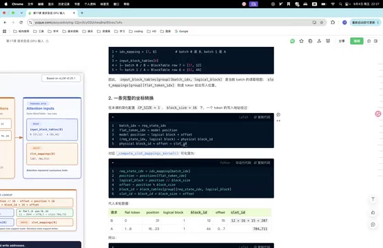
The complete conversion pipeline:
batch_index → request_state_index (via index_mapping)
flat_token_index → position (one-to-one correspondence)
position → logic_block + offset (division and modulo)
request_state_index + logic_block → physical_block_id (block_table lookup)
physical_block_id + offset → slot_id (final physical address)
The essence of this pipeline is linearizing a two-dimensional (block, offset) coordinate into a one-dimensional address, similar to row-major storage of 2D arrays in C.
Address Calculation Example
Taking the first token of Request B as an example:
- flat_token_index = 0, position = 31
- logic_block = 31 // 16 = 1 (block_size=16, meaning each block holds KV Cache for 16 tokens)
- offset = 31 % 16 = 15 (the 16th slot within that block, zero-indexed)
- Look up block_table[7][1] = 12 (Request B's second logical block maps to physical block 12)
- slot_id = 12 * 16 + 15 = 207 (global physical slot number)
Note that the slot_id unit is not bytes but rather a KV Cache unit, as defined by the attention banking mechanism. The actual byte size of each KV Cache unit depends on the model's head_dim and data precision — for example, with FP16 precision and head_dim=128, a single slot stores one pair of KV vectors requiring 2 × 128 × 2 = 512 bytes (multiplied by the number of attention heads). Different KV Cache groups generate their own block_tables and slot_mappings. The concept of KV Cache groups originates from techniques like GQA (Grouped Query Attention) — in GQA, multiple query heads share the same set of KV heads, so different head groups may correspond to independent KV Cache storage regions that require separate physical block allocation management.
Complete Input Preparation for the Attention Module
After the above conversions, the worker has prepared the complete input for attention computation. Modern efficient attention implementations (such as FlashAttention and FlashInfer) require inputs to strictly conform to specific memory layout specifications to fully leverage GPU shared memory and register hierarchies for optimal computational performance.
input_batch contains:
- request_id list
- index_mapping (batch index to global index mapping)
- input_ids (actual token sequence)
- position array (token position information, used by positional encoding schemes like RoPE)
- query_start_loc (request boundary markers, ensuring attention does not leak across requests)
- seq_lens (sequence length of each request, including both historical and newly added tokens; the attention kernel uses this to determine the KV range each query token should attend to)
Each KV Cache group provides:
- input_block_tables (list of visible physical blocks; the kernel uses indirect addressing to access KV Cache blocks scattered across GPU memory, achieving efficient zero-copy random access)
- slot_mapping (write location mapping table, specifying the target slots for newly generated KV vectors)
These data structures form the input format that the GPU can directly consume, and the attention kernel performs efficient parallel computation based on them.
Summary of the Four Index Space Mappings
vLLM's scheduling and execution involves four key index spaces:
- request_state_index: The row number of a request in the worker's global state, used to persistently store computation progress and the block_table. Its lifecycle spans from request arrival to request completion.
- batch_index: The row number of a request in the current batch — a compact index temporarily generated for each step, linked to request_state_index via index_mapping.
- flat_token_index: A token's position in the flattened sequence — the global index after concatenating tokens from multiple requests into a one-dimensional contiguous array.
- position: A token's position in the original request sequence, reflecting the token's true ordinal number within the full conversation/generation context.
These four index spaces form a complete mapping chain from high-level semantics to low-level physics: request_state_index and batch_index handle request-level management, flat_token_index achieves the contiguity required for GPU computation, and position connects to the physical addressing of KV Cache. Understanding these index spaces and their transformation relationships is fundamental to deeply comprehending vLLM's architecture. It is recommended to work through the example diagrams repeatedly to master the complete mapping path from CPU scheduling instructions to GPU physical addresses.
Key Takeaways
Related articles

AI Training Facilities Face Superhuman Hacker Threats: An Unprecedented Cybersecurity Risk
AI safety experts warn: next-gen LLM training infrastructure may face superhuman-level attacks from AI hackers, with threat scales exceeding all of human history.

Anthropic Employee Resignation Sparks Deep Discussion on AI Industry Talent Mobility
An Anthropic employee's public resignation sparked heated debate on Hacker News. Analyzing AI talent mobility, technical direction disputes, cultural shifts, and the commercialization challenges facing AI safety companies.

Querit Search API: Real-Time Search and Scheduled Monitoring for AI Agents
Querit is a web search API for LLMs and AI Agents with millisecond response times, Monitor API for scheduled tracking, multi-source deduplication, Dify/LangChain integration, and 83.17% FreshQA accuracy.