Deep Dive into vLLM Worker-Side GPU KV Cache Initialization
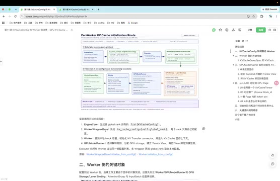
How vLLM Workers allocate and bind GPU KV Cache from logical blocks to physical memory.
This article provides a deep analysis of vLLM's Worker-side KV Cache initialization, tracing the full path from KVCacheConfig generation to physical GPU memory allocation. It covers how ModelRunner allocates untyped byte arrays, reshapes them into KV Cache tensor views via zero-copy, and binds them to attention layers. A concrete example illustrates the multi-level mapping from logical blocks to physical memory positions.
In vLLM's inference engine, KV Cache management is the core mechanism that determines GPU memory utilization and throughput.
KV Cache Technical Background
KV Cache (Key-Value Cache) is a fundamental technique for accelerating Transformer model inference. During autoregressive generation, producing each new token requires the Key and Value vectors of all preceding tokens. Recomputing these every time would introduce massive redundant computation. KV Cache addresses this by caching previously computed Key-Value pairs, so that each step only needs to compute the KV for the new token and concatenate it with the cache. This technique reduces inference time complexity from O(n²) to O(n), but at the cost of significant GPU memory consumption. For a typical LLaMA-70B model processing 4096 tokens, the KV Cache can occupy tens of gigabytes of GPU memory, making efficient KV Cache memory management a core challenge for inference systems.
In previous discussions, we explored how KVCacheConfig is generated and how it is consumed by the SchedulerConnector on the scheduling side (AsyncLLM/EngineCore) to establish logical block pools and block tables. However, all of that is logical-level abstraction — the actual physical GPU memory allocation happens on the Worker side.
This article focuses on how KVCacheConfig is consumed on the Worker side: how Workers actually allocate KV Cache tensors on the GPU based on the configuration, and how logical blocks are mapped to physical memory locations.
The Propagation Path of KVCacheConfig
From generation to consumption by Workers, KVCacheConfig traverses a relatively long call chain. The entire process can be broken down into several key stages.
vLLM Architecture and Separation of Concerns
vLLM adopts a classic scheduling-execution separation architecture. The scheduling side (EngineCore/AsyncLLM) handles request management, sequence scheduling, and logical resource allocation. It maintains logical-level block tables and decides which requests should be processed and how many resources they need. The execution side (Worker) handles actual model inference and physical memory management. This separation brings multiple benefits: scheduling logic is decoupled from hardware, enabling support for various backends; the scheduler can perform global optimization without knowing GPU details; and Workers can focus on efficient execution. The two sides communicate via RPC — the scheduler dispatches execution commands, and Workers return results. This architecture is especially important in distributed inference scenarios, where the scheduler needs to coordinate the work of multiple GPU Workers.
During the Worker startup phase, it goes through init_worker, init_device, model loading, profiling, and projection steps. After that comes the KV Cache initialization phase, which starts from EngineCore.
After collecting model and hardware information from each GPU and each Worker, EngineCore constructs a list of KVCacheConfig — note that it's a list, with each element corresponding to the configuration for a specific Worker. This list is then passed to WorkerWrapperBase via an RPC call.
The Concept of Rank in Distributed Inference
In multi-GPU distributed training or inference, each process/device has a unique identifier. The global_rank is the process's global index across the entire cluster (e.g., 0 to 15), while local_rank is the process's index within a single machine (e.g., 0 to 7). These indices are used to: determine which model shard a process should load (model parallelism), assign data partitions (data parallelism), select which GPU device to use, and identify roles in collective communication. In vLLM, EngineCore generates a configuration list for all Workers, with each element corresponding to one Worker. WorkerWrapperBase extracts its own configuration from the list based on its global_rank, so each Worker knows how much KV Cache it should manage and which resources to use. This design allows the same code to run on different Workers, differentiated only by rank.
The key point is that WorkerWrapperBase selects its own local config from the entire configuration list based on the current global_rank. This step narrows down from "global configuration" to "local configuration," after which the actual initialization work is handed off to the Worker.
Four Core Stages
The entire Worker-side initialization can be summarized in four stages:
- EngineCore generates the KVCacheConfig list
- WorkerWrapperBase selects its own Config by rank
- Worker performs preliminary initialization and sets the block count
- GPUModelRunner executes the actual memory allocation and binds KV Cache to the model
As you can see, the Worker itself acts more as a "resource orchestrator," while the real work of physical allocation is performed by its ModelRunner.
Responsibilities of Each Layer and Data Structures
Understanding this mechanism requires clarifying the responsibilities of several key structures.
Composition of KVCacheConfig
KVCacheConfig is essentially a "resource contract" for the current Worker, consisting of three main parts:
- num_blocks: The number of available blocks — fairly self-explanatory.
- KVCacheGroups (KVCacheGroupSpec): Describes which layers share the same logical block table, expressing logical ordering and cache strategy grouping.
- KVCacheTensors (KVCacheTensor): Primarily used by Workers, describing the physical storage slots allocated by the Worker, with fields identifying specific GPU memory locations.
Hybrid Attention Mechanisms
Modern large models often employ hybrid attention architectures to balance performance and efficiency. Full Attention lets each token attend to all historical tokens, capturing long-range dependencies but with high computational cost. Sliding Window Attention only attends to the most recent tokens (e.g., 4096), reducing computational complexity. Group Query Attention (GQA) allows multiple query heads to share the same set of KV pairs, reducing KV Cache size. Different layers of a model may use different attention mechanisms: lower layers use Full Attention to capture global semantics, while upper layers use Sliding Window for efficiency. This hybrid design poses challenges for KV Cache management: different layers require different Cache sizes and access patterns, necessitating a unified abstraction for management. vLLM addresses this through a Group mechanism that groups layers using the same attention strategy, with each group sharing a logical block table, elegantly supporting hybrid architectures.
There's a particularly confusing point worth emphasizing: layers within the same Group are typically distributed across different Tensors; while layers from different Groups but in the same slot may actually reside in the same Tensor. This design specifically supports hybrid attention layouts, which we'll illustrate with a concrete example later.
Collaboration Between Worker and ModelRunner
The Worker holds a ModelRunner, which is the actual "assembler." ModelRunner is responsible for:
- Managing
KVCacheAttentionGroup(the input grouping for KV Cache) - Executing physical Tensor allocation
- Performing type conversion — transforming untyped byte arrays into KV Cache views specific to the model
- Binding the final Tensor views to Attention layers
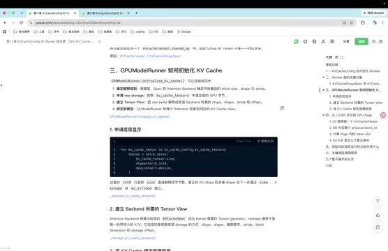
Once binding is complete, Attention layers can directly access their corresponding KV Cache tensor views for reads and writes during inference.
ModelRunner's Memory Allocation Process
ModelRunner's initialization is divided into three main steps: determining interpretation rules (initializing helper classes like banking), executing memory allocation, and performing type conversion with model binding.
Step 1: Physical Allocation
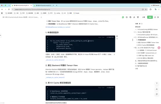
The actual memory allocation logic iterates through KVCacheTensor entries and allocates them one by one. Interestingly, allocation uses the int8 data type — meaning vLLM actually allocates an untyped byte array on a per-byte basis. This design provides tremendous flexibility.
Step 2: View Transformation (reshape)
Tensor Views and Zero-Copy Technique
In deep learning frameworks, the reshape operation on a Tensor is a zero-copy technique. The physical data layout in GPU memory remains unchanged — only the way the data is interpreted changes, i.e., the dimensions, strides, and other metadata are modified. For example, a one-dimensional array of shape [1024] can be reshaped into a [32, 32] two-dimensional matrix, but the underlying 1024 numbers remain in exactly the same positions in memory. This allows the same block of memory to be interpreted in multiple ways: as a byte array during allocation for convenient memory management and alignment, and as a specifically shaped Tensor during model computation. vLLM leverages this property by first allocating GPU memory as int8 byte arrays (for precise byte-level size control), then reshaping them into multi-dimensional Tensors matching the actual KV Cache dimension requirements. The entire process involves no data copying whatsoever — both flexible and efficient.
After allocating the byte arrays, ModelRunner performs a reshape operation on them according to KVCacheSpec. Reshape only changes the interpretation of the storage — how these bytes are read — and does not require reallocating memory. This is an extremely lightweight and efficient operation.
Step 3: Binding to the Model
After completing the view transformation, the Tensor references (pointers) are placed in two locations:
ModelRunner's KV Cache container- The forward pass context
This way, Attention layers can directly use these Tensor Views during forward computation.
From Logical to Physical Positions: A Complete Example
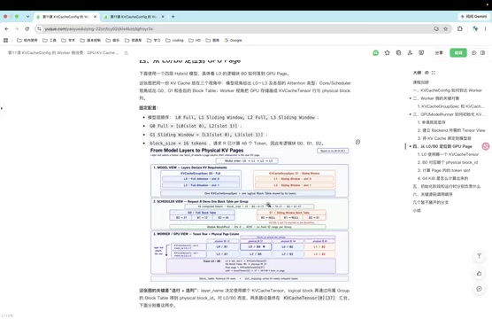
The most elegant part of this entire mechanism is how it connects three perspectives: the "model view," the "scheduler view," and the "GPU physical view." Let's use a concrete example to illustrate.
Model View: Grouping
Assume a model has 4 layers: L0, L1, L2, L3. After grouping:
- Group0: L0, L2 — using Full Attention
- Group1: L1, L3 — using Sliding Window Attention
Within Group0, L0 is at Slot0 and L2 is at Slot1; L1 and L3 are similarly distributed within Group1. A KVCacheGroupSpec expresses that these layers share the same logical block table.
Scheduler View: Logical Resource Allocation
PagedAttention and Block Management
One of vLLM's core innovations is borrowing the virtual memory management concept from operating systems to organize KV Cache into fixed-size blocks (similar to memory pages). Each block typically contains KV data for 16 or 32 tokens. This design brings three major advantages: First, it enables non-contiguous physical storage, avoiding memory fragmentation. Second, it allows sharing identical KV Cache blocks across different sequences (e.g., common prompt prefixes), significantly improving memory utilization. Third, it supports dynamic block allocation and deallocation, similar to OS page swapping. The scheduler maintains a mapping table from logical blocks to physical blocks (block table), just like a page table. This design enables vLLM to support larger batch sizes with the same amount of GPU memory, thereby significantly improving throughput.
From the scheduler's perspective, a Manager is generated for each Group to handle logical resource allocation. Suppose at a given moment 48 tokens have been computed and the block size is 16 — then 3 logical blocks are needed to hold these tokens.
Physical View: Two KVCacheTensors
The key lies in the two KVCacheTensors created during allocation:
- Tensor0: Stores all layers corresponding to Slot0, i.e., L0 from Group0 and L1 from Group1
- Tensor1: Stores all layers corresponding to Slot1, i.e., L2 and L3
This confirms the "counterintuitive" conclusion mentioned earlier: layers from different Groups but the same Slot are placed in the same Tensor.
Coordinate Positioning: Row and Column Mapping
Block Table Multi-Level Mapping Mechanism
The block table implements multi-level mapping from logical to physical positions. The first level is the sequence level: each generation sequence has its own logical block list, indicating which logical blocks the sequence occupies (e.g., [0, 1, 2] means the first 3 blocks). The second level is the Group level: each attention group maintains a GroupBlockTable that maps logical block IDs to physical block IDs (e.g., logical block 0 → physical block 37). The third level is the Tensor level: based on the layer's slot, it determines which KVCacheTensor to use; then based on the physical block ID and token offset, it calculates the exact offset address within that Tensor. This multi-level mapping enables flexible resource management: the scheduler only needs to operate on logical blocks while Workers handle the mapping to physical memory; different sequences can share the same physical blocks (prefix sharing); and physical blocks can be dynamically allocated and reclaimed.
Each Tensor is a long tensor, and locating a specific KV Cache entry requires determining both the "row" and "column":
Determining the row (which Tensor + position within the layer): Based on the layer name, determine which Group and which Slot the layer belongs to. For example, L0 belongs to Group0's Slot0, so its data resides in Tensor0.
Determining the column (physical block position): Through the mapping chain: logical block → GroupBlockTable → physical_block_id. Suppose the scheduler assigns a physical_block_id of 37 to a logical block — this locates the column position at the 37th block in the Tensor.
Pinpointing the Token Slot
After finding the block, we still need to calculate the specific Token Slot within the block. Take the 7th token as an example (with a block size of 16):
- Logical block index = 7 // 16 = 0
- Token offset = 7 % 16 = 7
The final physical address is calculated as: Tensor0 base address + 37 × 16 + 7. That is, first locate Tensor0, skip the first 37 blocks, then offset by 7 token positions to precisely reach the target KV Cache's physical storage location.
This conversion chain of model grouping → physical resources → logical positions → GPU physical locations achieves the decoupling of logic and physics in a remarkably elegant way.
Initialization Phase vs. Runtime Phase
Finally, it's important to distinguish the responsibilities of each phase:
Initialization Phase (Static):
- Complete GPU memory allocation
- Determine Tensor views (reshape)
- Bind Tensors to fixed layers
- Determine the number of available blocks
Runtime Phase (Dynamic):
- Block table contents for each Group change dynamically (e.g., mappings like [37, 12, 44] are continuously updated)
- Current token positions change
- Actual KV Cache contents change
- Block reference counting and reuse (efficient cache reuse)
Summary
After initialization is complete, model layers are bound to their KV Cache views. At runtime, the block table maps logical block indices to physical block IDs, and combined with slot mapping and token offsets, the exact physical slot for writing is determined.
The elegance of this design lies in: using untyped byte arrays for underlying allocation, using reshape for zero-copy view transformation, and using the grouping mechanism to uniformly manage heterogeneous attention layers — achieving efficient GPU memory management while maintaining flexibility. Although the actual code implementation is quite complex, the abstracted core logic is clean and elegant, well worth deep study by any developer interested in inference engines.
Key Takeaways
- KV Cache management is critical to vLLM's inference performance, involving a sophisticated interplay between logical abstraction and physical implementation
- Configuration flows from EngineCore through WorkerWrapperBase (distributed by rank), with ModelRunner ultimately performing physical allocation
- The byte array + reshape zero-copy technique is both flexible and efficient
- The Group mechanism supports hybrid attention architectures, with layers from different groups but the same slot sharing physical Tensors
- Multi-level mapping (logical block → physical block → Tensor offset) achieves decoupling between scheduling and execution
- The initialization phase establishes static structures, while the runtime phase dynamically updates block mappings
Related articles
How Much Does CPU Performance Actually Matter for Pure GPU Inference?
Analysis of CPU's real impact in pure GPU inference: from tokenization to decoding. Learn why GPU budget matters more than CPU for local AI deployment.

Zepto Builds AI Customer Service with MLflow: An Evaluation-Driven Practice Guide
Deep dive into how Zepto built an evaluation-driven AI customer service system using MLflow and Databricks, achieving 60% faster responses and 40% less manual handling. From technical architecture to practical insights.
Iran Captures U.S. Underwater Drone in Strait of Hormuz: A Comprehensive Analysis
Iran announces capture of U.S. Navy underwater drone in Strait of Hormuz. In-depth analysis of the incident, strategic value of UUVs, U.S.-Iran geopolitical competition, and implications for global energy security and military dynamics.