From Matrix Algebra to JAX: Building Neural Networks by Hand to Understand the Essence of Deep Learning

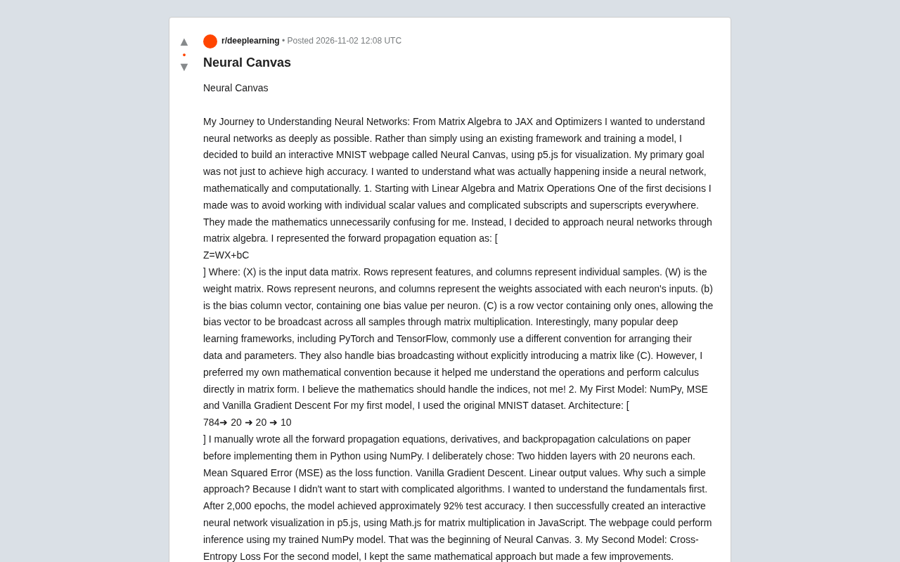
Most people start learning about neural networks by calling libraries: run model.fit(), watch the accuracy go up, and call it done. But one developer on Reddit took a different path—MuhammadEssa hand-wrote forward propagation, backpropagation, and gradient descent in NumPy, then rewrote it in JAX, and finally built an interactive MNIST visualization web page called Neural Canvas. The core motivation behind the whole process wasn't chasing high accuracy, but figuring out what the network is actually computing internally.

Recasting Forward Propagation with Matrix Algebra

The developer's first decision was to abandon scalar notation. Traditional tutorials are full of $w_{ij}^{(l)}$ and $b_j^{(l)}$, and he felt the math was drowning in subscripts. He switched to expressing forward propagation in matrix form: Z = WX + bC, where each column of X is a sample, each row of W corresponds to a neuron, b is the bias column vector, and C is an all-ones row vector that broadcasts the bias across all samples via matrix multiplication.

He specifically notes that PyTorch and TensorFlow use a different convention—they typically place samples along the rows, and bias broadcasting is handled implicitly by the framework, so there's no need to explicitly construct the C matrix. But he stuck with his own convention for a very practical reason: this arrangement let him do calculus derivations directly in matrix form without manually tracking every index. In his words, "the math should handle the subscripts, not me."

This choice itself reflects a learning strategy: rather than accommodating the framework's default habits, pick the mathematical convention that makes derivation easiest for you, and once you understand it thoroughly, adapt to engineering conventions later.

Matrix Calculus is the key tool here. Traditionally, network gradients are derived element by element using the scalar chain rule, but when parameters are organized as matrices, differentiating directly with respect to matrices keeps expressions concise. For example, if the loss function is a scalar L and Z = WX + bC, then ∂L/∂W takes the form (∂L/∂Z) · Xᵀ, where the bias gradient requires summing over all samples. These "matrix-by-matrix" differentiation rules (often using denominator layout or numerator layout) keep backpropagation derivations from drowning in subscripts. The author's insistence on arranging samples by column and broadcasting bias with an all-ones row vector is precisely so these gradient formulas can be written in a single line on paper, keeping attention on the structure of the chain rule rather than shuffling indices.

Four Models, a Step-by-Step Learning Path of Increasing Difficulty

First Model: NumPy + MSE + Naive Gradient Descent

He built a 784→20→20→10 network using the original MNIST dataset, hand-derived all forward propagation equations, derivatives, and backpropagation on paper, then implemented it in NumPy. The loss function was mean squared error (MSE), the optimizer was the most naive gradient descent, and the output layer had no activation function. After training for 2000 epochs, test accuracy was about 92%.

The focus at this stage wasn't performance but verifying whether his understanding of the chain rule was correct. He then built a web-based inference visualization using p5.js and Math.js—that's where the prototype of Neural Canvas came from.

Second Model: Switching to Cross-Entropy Loss

The architecture expanded to 784→40→40→10, MSE was replaced with cross-entropy, softmax was added to the output layer, and the optimizer remained naive gradient descent. After 2000 epochs, accuracy was about 96%. By this point, he began to feel he was understanding the network rather than copying code from a tutorial.

The combination of cross-entropy loss and softmax is the standard configuration for classification tasks. Softmax converts network outputs into a probability distribution: for each sample, take the exponential of the logits and normalize so that the probabilities across classes sum to 1. Cross-entropy then measures the difference between the predicted distribution and the true one-hot label, in the form -Σ yᵢ log(ŷᵢ). Compared to MSE, cross-entropy penalizes wrong predictions more steeply, and when combined with softmax, the gradient takes a very clean form: ∂L/∂z = ŷ - y, which avoids the vanishing gradient problem MSE has when the output layer saturates. The author introduced this combination in the second model, which not only improved accuracy but also made backpropagation derivations clearer—the output layer error is simply the difference between predicted probabilities and true labels.

Third Model: JAX Takes Over Automatic Differentiation

When he wanted to try three hidden layers, he hit a practical problem: manually deriving the derivatives and chain rule for each layer was too time-consuming. So he turned to JAX, developed by Google, using its automatic differentiation to directly compute gradients of the loss function with respect to parameters, including entire weight matrices.

The model used the Arabic Digits MNIST dataset with architecture 784→20→20→15→10, cross-entropy loss plus naive gradient descent, reaching about 96% accuracy after 2000 epochs. His exact words were that he "really fell in love with JAX"—the derivation time saved let him focus on mathematical understanding and architecture experiments.

JAX's automatic differentiation is based on the functional programming paradigm, transforming pure functions via jax.grad to return their gradient functions. It supports both forward-mode and reverse-mode automatic differentiation; for the gradient of a scalar loss with respect to a large number of parameters in neural networks, reverse mode (i.e., backpropagation) is the efficient choice. What's unique about JAX is that it uses jit compilation and vmap automatic vectorization, transparently extending gradient computation across the entire parameter matrix without manually writing loops. Unlike PyTorch's dynamic graph, JAX requires functions to be side-effect-free, which makes gradient computation more predictable. After replacing manual chain rule with JAX, the author could easily try three hidden layers, because no matter how deep the network, jax.grad automatically provides the correct gradients, eliminating the tedium of layer-by-layer derivation.

Fourth Model: The Efficiency Leap from Momentum

The fourth model switched to the Persian Digits MNIST dataset with the same architecture as the third. The original plan was to go straight to Adam, but he realized that understanding Adam requires grasping several prerequisite concepts first, so he stepped back and implemented mini-batch gradient descent with momentum using JAX.

The result was unexpected: about 96% test accuracy in roughly 200 epochs, whereas previously reaching a similar level required about 2000 epochs. This comparison gave him an intuitive sense of how much optimization algorithms affect training efficiency—under his experimental conditions, convergence speed improved by an order of magnitude.

Momentum is an improvement on naive gradient descent, designed to accelerate convergence and suppress oscillations. It introduces a velocity variable v that accumulates historical gradients: v = βv + (1-β)∇θL, then updates parameters as θ = θ - αv, where β is typically 0.9. Intuitively, momentum accelerates parameters in dimensions where the gradient direction is consistent and decelerates them in dimensions where the gradient direction keeps changing, thereby moving faster through flat regions and narrow valleys. Combined with mini-batch (estimating gradients from a small batch of samples each time), training becomes both stable and efficient. The author observed an order-of-magnitude improvement in convergence speed precisely because momentum effectively leverages historical gradient information, while the noise introduced by mini-batch in each update also helps escape local minima. This lays the foundation for understanding Adam later (which combines momentum and adaptive learning rates).

Learning Roadmap and Core Advice

He hasn't built the fifth model yet, but the roadmap is set: first implement mini-batch gradient descent with RMSProp, then Adam, then move on to convolutional neural networks. His principle is to mathematically understand and personally implement each optimization algorithm before moving to the next.

His advice for beginners is straightforward: start with linear algebra, and don't jump straight into advanced architectures, optimizers, or high-level frameworks. You don't need to master every mathematical concept before getting hands-on, but at least thoroughly understand matrix multiplication and how it represents the operations inside a network. His summary: don't just train neural networks, understand them.

The project is open-sourced on GitHub (MuhammadEssa2002/neural_canvas) and offers an online demo where you can directly observe the network's inference process in your browser.

Is This Approach Worth Learning?

From an engineering efficiency standpoint, hand-deriving gradients and then writing a NumPy implementation is clearly not cost-effective—a single line of jax.grad solves it. But from a learning perspective, the manual derivations in the first two models build muscle memory for backpropagation, and that understanding pays off when debugging training anomalies or designing custom loss functions.

A more pragmatic compromise is: first hand-write the backpropagation for a two-layer network to build intuition, then use JAX's automatic differentiation for experiments, but define the model structure, loss function, and parameter update rules yourself at every step rather than directly calling model.compile(). The Neural Canvas path roughly follows this approach—the first two models lay the foundation, and the latter two use tools to accelerate, without compromising depth of understanding.

One-line Summary

Developer hand-writes neural networks in NumPy and JAX, deepening understanding of internal math through four progressive models.

Paragraph Summary

To truly understand the internal operations of neural networks, a developer abandoned calling libraries and hand-wrote forward propagation, backpropagation, and gradient descent in NumPy, using matrix form Z=WX+bC to simplify derivations. He built four progressively upgraded models: from NumPy+MSE at 92% accuracy, to cross-entropy+softmax at 96%, then to deeper networks with JAX automatic differentiation, and finally using momentum-based mini-batch to reduce convergence from 2000 to 200 epochs. The whole process emphasizes mathematical understanding over chasing scores, and offers a learning roadmap starting from linear algebra and hand-implementing optimizers. The project is open-sourced as the Neural Canvas interactive visualization web page.