Quantization Illustrated: A Deep Dive into Core Compression Techniques for Large Language Models

Why Large Language Models Need Quantization

As large language models (LLMs) continue to grow from billions to hundreds of billions of parameters, their storage and inference costs have skyrocketed. A model with 70 billion parameters, stored in 32-bit floating point (FP32), requires approximately 280GB of memory for weights alone—far exceeding the VRAM capacity of most consumer-grade or even professional GPUs.

More importantly, the performance bottleneck for LLM inference often isn't compute power, but memory bandwidth. During autoregressive generation, every single token generated requires loading all model weights from VRAM, making the inference process severely memory-bandwidth bound. Take the NVIDIA A100 as an example: with a memory bandwidth of 2TB/s, loading a 280GB FP32 model takes approximately 140ms—meaning weight loading alone limits generation to roughly 7 tokens per second. Therefore, reducing model size isn't just about saving space; it's the key to directly improving inference speed.

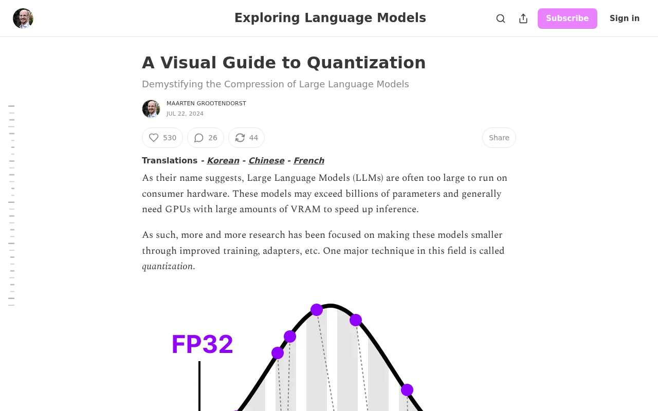
Quantization is the core technique born to solve this exact challenge. Its fundamental idea is intuitive: use lower-precision numerical representations to store and compute model parameters, thereby dramatically reducing memory footprint and computational overhead within an acceptable range of precision loss. Quantization is one of the key engineering techniques that makes large models actually runnable and affordable.

What Is Quantization: Mapping from High Precision to Low Precision

The Essence of Numerical Precision

In deep learning, model weights are typically stored as floating-point numbers. To understand quantization, you first need to understand the internal structure of these numerical formats. According to the IEEE 754 standard, floating-point numbers consist of three components: the sign bit (positive/negative), exponent bits (determining the value range), and mantissa bits (determining precision). Common precision formats include:

• FP32 (32-bit floating point): 1 sign bit + 8 exponent bits + 23 mantissa bits. Standard precision, with each parameter occupying 4 bytes. Offers extremely high numerical precision and a dynamic range of approximately ±3.4×10³⁸.
• FP16 (16-bit floating point): 1 sign bit + 5 exponent bits + 10 mantissa bits. Half precision, with each parameter occupying 2 bytes. Has a smaller dynamic range (approximately ±65504) and is prone to numerical overflow when training large models.
• BF16 (Brain Floating Point 16): 1 sign bit + 8 exponent bits + 7 mantissa bits, proposed by the Google Brain team. It retains the same exponent width as FP32 (thus maintaining the same dynamic range) while sacrificing mantissa precision. This makes BF16 particularly well-suited for deep learning training, since neural networks need dynamic range far more than precision.
• INT8 (8-bit integer): Each parameter occupies only 1 byte, representing 256 discrete values.
• INT4 (4-bit integer): Each parameter occupies only 0.5 bytes, representing 16 discrete values.

The core of quantization is "mapping" high-precision floating-point values to a lower-precision representation space. For example, going from FP32 to INT8 can theoretically compress the model to one-quarter of its original size, while INT4 can compress it to one-eighth.

The Mathematical Principles of Quantization Mapping

The key to quantization lies in how to map a continuous range of floating-point numbers to a discrete range of integers. This process typically relies on two parameters: the scale factor and the zero-point.

Taking symmetric quantization as an example, we first determine the value range of the weights (maximum absolute value), then compute a scale factor to linearly map float values to an integer interval (e.g., INT8's -127 to 127). The specific formula is:

q = round(x / s)

Where x is the original floating-point value, s is the scale factor (s = max(|x|) / 127), and q is the quantized integer value. During dequantization, the approximate floating-point value is recovered via x̂ = q × s.

This mapping inevitably introduces precision loss—essentially a form of quantization noise. From a signal processing perspective, the error introduced by uniform quantization approximately follows a uniform distribution, with variance Δ²/12 (where Δ is the quantization step size). The larger the step size (i.e., the lower the bit count), the greater the noise.

In practice, the granularity of quantization significantly impacts precision. Common granularity choices include:

• Per-tensor quantization: The entire weight matrix shares a single scale. Simplest to implement but offers the worst precision.
• Per-channel quantization: Each output channel uses an independent scale, substantially improving precision.
• Per-group quantization: Channels are further subdivided into fixed-size groups (e.g., 128 elements per group), with each group quantized independently. This is the mainstream choice for current INT4 quantization.

Finer granularity allows the scale to better adapt to local value distributions, reducing quantization error, but it also increases the overhead of storing additional scale parameters. Current mainstream 4-bit quantization schemes (such as GPTQ and AWQ) commonly adopt a per-group quantization strategy with group size=128.

Comprehensive Analysis of Mainstream Quantization Methods

Differences Between Symmetric and Asymmetric Quantization

Symmetric quantization assumes the value distribution is centered symmetrically around zero, with the zero-point fixed at 0. It's simple to compute and efficient, but wastes representation space when the data distribution is asymmetric. For example, if weights range from [-1, 10], symmetric quantization would use [-10, 10] as the mapping range, wasting much of the negative number interval.

Asymmetric quantization allows a shifted zero-point, enabling more precise coverage of the actual value distribution range, at the cost of slightly more complex computation (requiring additional zero-point offset handling in matrix multiplication). In practice, weights tend to have approximately symmetric distributions suited for symmetric quantization, while activations—which tend to shift after passing through nonlinear functions like ReLU (often concentrated in the positive region)—are better suited for asymmetric quantization.

Post-Training Quantization (PTQ): Low-Cost Rapid Deployment

Post-training quantization is currently the most commonly used quantization approach. It directly quantizes weights after model training is complete, without requiring retraining. The advantage of PTQ lies in its low cost and fast implementation, making it suitable for rapid deployment. Representative methods include:

GPTQ: Efficient Layer-wise Quantization Based on Second-Order Information

GPTQ (2022) is one of the most influential PTQ methods today. Its technical lineage traces back to classical neural network pruning theory: Optimal Brain Damage (OBD, 1989) used diagonal approximations of the Hessian matrix to assess weight importance; Optimal Brain Surgeon (OBS, 1993) further considered correlations between weights, using the full Hessian inverse to optimally adjust remaining weights after pruning.

GPTQ extends the OBS framework from pruning to quantization: when a weight is quantized (introducing error), it uses the Hessian inverse to optimally adjust the not-yet-quantized weights in the same row, thereby compensating for quantization error. To make this process feasible for models with tens of billions of parameters, GPTQ introduces a key engineering optimization—efficiently updating the Hessian inverse via Cholesky decomposition and processing weights in column-order batches, allowing the entire quantization process to be completed on a single GPU within hours.

AWQ: Activation-Aware Weight Quantization

AWQ (Activation-aware Weight Quantization, 2023) presents a seemingly counterintuitive but highly effective insight: protecting just 1% of salient channels from quantization can dramatically reduce overall quantization loss. Here, "salient" is determined not by the absolute magnitude of the weights themselves, but by the magnitude of the corresponding input activations—if a particular input channel has large activation values, even small-magnitude weights in that channel will have their quantization errors amplified and propagated.

However, directly keeping some weights in higher precision causes hardware inefficiency due to mixed precision. The elegance of AWQ lies in finding an equivalent transformation: by multiplying the weights of salient channels by a scaling factor greater than 1 (while dividing the input by the same factor to maintain mathematical equivalence), the relative quantization error for these weights is significantly reduced. This method achieves effects close to mixed-precision protection without introducing any mixed-precision overhead.

These methods maintain good model performance at INT4 precision through clever calibration strategies.

Quantization-Aware Training (QAT): High-Precision Guarantee

Quantization-aware training simulates quantization-induced errors during the training process, allowing the model to "adapt in advance" to low-precision environments. In practice, "fake quantization" nodes are inserted during forward propagation to simulate the noise introduced by the quantization-dequantization process; during backward propagation, since the rounding operation is non-differentiable, the Straight-Through Estimator (STE) is typically used to approximate gradients, passing the gradient of the quantization node directly to the previous layer.

Compared to PTQ, QAT typically achieves higher precision, with particularly notable advantages in ultra-low-bit scenarios (such as INT4 or lower). However, it requires retraining the model, which is computationally expensive (typically requiring 1-10% of the original training compute), making it more suitable for scenarios with strict precision requirements. Recently, Meta's SpinQuant and Qualcomm's QuIP# have attempted to combine rotation transformations with QAT principles, achieving remarkable results at ultra-low bit widths.

Core Challenges Facing Quantization

The Outlier Problem and Solutions

A thorny issue in large model quantization is outliers. Research has found that a small number of extremely large "outlier features" exist in LLM activations, significantly expanding the numerical range and causing quantization precision to drop sharply.

These outliers don't appear randomly—they have structural causes. Research shows (Dettmers et al., 2022) that in Transformer models, specific hidden dimensions persistently exhibit abnormally large activation values across all tokens and all layers, and this phenomenon becomes more pronounced as model scale increases (beyond 6.7B parameters). The root cause is related to the cumulative effects of attention mechanisms and residual connections—certain dimensions are continuously amplified during layer-to-layer propagation, forming "fixed outlier channels."

Several solutions have been proposed:

• LLM.int8() (Dettmers et al., 2022): Employs a mixed-precision decomposition strategy—identifying outlier dimensions through threshold detection (typically only 0.1% of dimensions), retaining FP16 precision for these dimensions while using INT8 quantization for the rest. Although it introduces additional branching logic, it achieves nearly lossless INT8 inference on 175B parameter models.

• SmoothQuant (Xiao et al., 2023): Proposes a more elegant approach—since outliers appear in activations rather than weights, a mathematically equivalent scaling transformation can "migrate" the quantization difficulty from activations to weights. Specifically, it introduces a per-channel smoothing factor that divides activation per-channel maximum values and multiplies the corresponding weight values, making the transformed activation distribution smoother and easier to quantize. This method avoids the hardware inefficiency of mixed precision.

• QuaRot (2024): Applies random orthogonal rotation transformations to weights and activations, "distributing" outlier energy across all dimensions, fundamentally eliminating the outlier problem.

The Precision-Efficiency Tradeoff

Quantization is fundamentally a game between precision and efficiency. The lower the bit count, the smaller and faster the model, but the greater the precision loss. Current research trends indicate:

• INT8 quantization: Can be achieved nearly losslessly and is the safest choice. Even with simple per-channel symmetric quantization, precision degradation is typically within 0.1%.
• INT4 quantization: Maintains usability when combined with advanced algorithms like GPTQ and AWQ, with perplexity increase typically between 0.5-1.0. This is the most mainstream deployment precision in the current community.
• INT3 quantization: Sits at the boundary of usability, requiring per-group quantization and advanced algorithms, with noticeable degradation possible on certain tasks.
• INT2 / INT1 (binarization): Still in the exploratory stage, with precision loss often unacceptable. Recent work like BitNet (Microsoft, 2024) attempts to train 1-bit models from scratch, bypassing the challenge of quantizing existing models and demonstrating an entirely new path.

Practical Value of Quantization

The significance of quantization technology extends far beyond "saving VRAM." It enables large models that could previously only run in data centers to be deployed on consumer GPUs, edge devices, and even smartphones, greatly expanding the application boundaries of large models. Additionally, smaller model sizes mean lower inference latency, less energy consumption, and lower operational costs.

Currently, quantization technology has developed a fairly mature toolchain and ecosystem:

• llama.cpp: A pure C/C++ inference framework developed by Georgi Gerganov that supports efficiently running quantized LLMs on CPUs. It defines the GGUF format (GPT-Generated Unified Format), supporting multiple quantization precisions from Q2 to Q8, and has become the de facto standard for local LLM deployment.
• vLLM: A framework focused on high-throughput GPU inference, supporting efficient serving deployment of quantized models like GPTQ and AWQ, achieving extremely high concurrency performance when combined with techniques like PagedAttention.
• TensorRT-LLM (NVIDIA): A deeply optimized GPU inference engine supporting INT8/INT4/FP8 quantization, achieving optimal hardware utilization through operator fusion and CUDA kernel optimization.
• Hugging Face Transformers: Through integration with libraries like bitsandbytes, auto-gptq, and autoawq, users can load quantized models with just one line of code (e.g., load_in_4bit=True).

On the model distribution side, community contributors like TheBloke (Tom Jobbins) on Hugging Face have provided pre-quantized versions for thousands of models, covering formats like GPTQ, AWQ, and GGUF, greatly lowering the barrier to entry for ordinary users.

Looking ahead, as quantization algorithms continue to evolve, future large models will become increasingly "lightweight" while maintaining their powerful capabilities. In particular, the FP8 format is already natively supported by NVIDIA H100/H200 GPUs and is poised to become the standard precision for next-generation training and inference. On the edge deployment front, chip manufacturers like Apple and Qualcomm are also adding hardware support for INT4 inference in their NPUs. For developers and researchers, understanding the principles and tradeoffs of quantization has become an essential foundation for effectively leveraging large models.

Summary

Quantization technology may seem complex, but it follows a clear logic: trade numerical precision for storage and computational efficiency, while using various clever algorithmic strategies to keep precision loss within acceptable bounds. From the choice between symmetric and asymmetric quantization, to the comparison of PTQ and QAT methods, to mixed-precision approaches for handling outliers—every step represents a crystallization of engineering and research wisdom. For those who wish to deploy large models with limited resources, mastering quantization technology is mastering the key to making AI accessible to all.

Key Takeaways