SAM 3 Auto-Labeling in Practice: Six Lessons Where Preprocessing Matters More Than the Model

Introduction: A Practical Summary That Could Save You Weeks

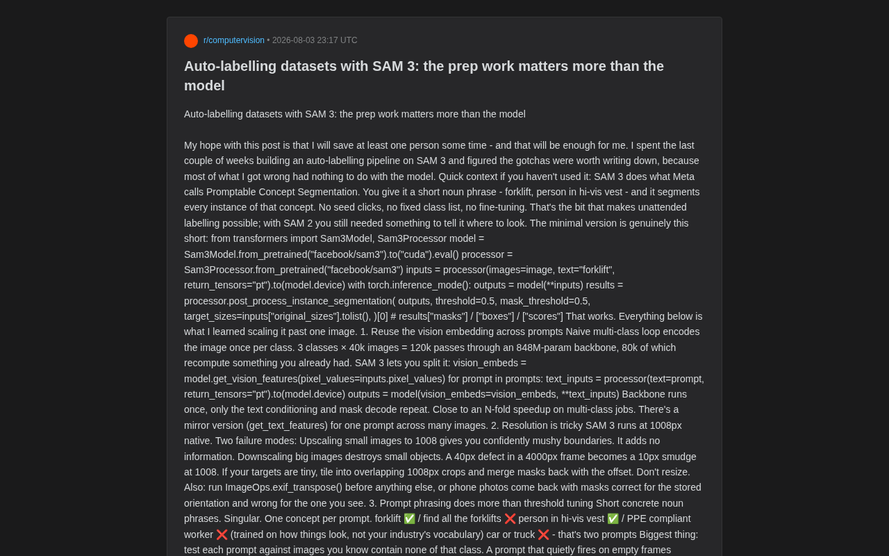
Recently, a developer shared their complete experience building an auto-labeling pipeline with Meta's latest segmentation model, SAM 3, on Reddit. After spending weeks scaling SAM 3 from a single-image demo to industrial-scale dataset annotation, they arrived at a counterintuitive conclusion: most of the pitfalls had nothing to do with the model itself—they were all about data preprocessing and engineering details.

This article systematically covers those practical lessons. If you're planning to use SAM 3 for large-scale data annotation, these "hard-won lessons" might help you avoid some costly detours.

SAM 3's Core Capability: Promptable Concept Segmentation

SAM 3 (Segment Anything Model 3) achieves what Meta calls Promptable Concept Segmentation. Its core breakthrough: you provide a short noun phrase—like "forklift" or "person in hi-vis vest"—and the model segments all instances of that concept in the image.

The Evolution of the SAM Series

To appreciate SAM 3's breakthrough, it helps to trace the series' development. SAM 1, released in 2023, introduced the "segment anything" concept, achieving zero-shot segmentation through interactive prompts (clicks, bounding boxes), but required manual spatial prompts to specify "where to segment." SAM 2 in 2024 extended capabilities to video, supporting temporal tracking and cross-frame propagation, but still relied on initial prompt points to initiate segmentation. SAM 3 introduces text-driven concept segmentation, completely eliminating the dependency on spatial prompts—a paradigm shift from "telling the model where to segment" to "telling the model what to segment." This is precisely the technical foundation that enables fully automated labeling pipelines.

This capability means:

• No seed clicks needed
• No fixed class list needed
• No fine-tuning needed

This is exactly what enables "unattended annotation." The author specifically noted that with SAM 2, you still needed some way to tell the model "where to look," while SAM 3 completely eliminates that constraint.

Technical Principles of Promptable Concept Segmentation

Architecturally, promptable concept segmentation leverages Vision-Language Alignment technology. The core architecture contains three key components: a vision encoder (typically based on ViT—Vision Transformer architecture, which splits images into patches and encodes them as high-dimensional feature vectors), a text encoder (a CLIP-like text understanding module that encodes natural language prompts into semantic vectors), and a mask decoder (which generates pixel-level segmentation masks guided by cross-attention between visual and text features). This architecture enables the model to understand concepts from an open vocabulary, rather than being limited to a fixed class list predefined during training—a fundamental difference from traditional closed-set segmentation models like Mask R-CNN.

SAM 3 Minimal Working Code

Getting started with SAM 3 requires surprisingly little code:

from transformers import Sam3Model, Sam3Processor

model = Sam3Model.from_pretrained("facebook/sam3").to("cuda").eval()
processor = Sam3Processor.from_pretrained("facebook/sam3")

inputs = processor(images=image, text="forklift", return_tensors="pt").to(model.device)
with torch.inference_mode():
    outputs = model(**inputs)
results = processor.post_process_instance_segmentation(
    outputs, threshold=0.5, mask_threshold=0.5,
    target_sizes=inputs["original_sizes"].tolist(),
)[0]
# results["masks"] / ["boxes"] / ["scores"]

This code does work. But the author emphasizes that the real challenge begins when you scale from one image to tens of thousands.

Six Engineering Lessons in Detail

Lesson 1: Reuse Vision Embeddings Across Prompts to Avoid Redundant Computation

The easiest performance mistake is re-encoding the image for every class in a multi-class loop. The author did the math:

3 classes × 40,000 images = 120,000 forward passes through an 848M-parameter backbone, of which 80,000 are redundantly recomputing what you already have.

The Computational Economics of Vision Embedding Reuse

This optimization is critical because modern Vision Transformers have computational complexity proportional to the number of input tokens (i.e., the square of resolution). With SAM 3's 848M-parameter backbone, visual encoding of a single 1008×1008 image may require tens of GFLOPS, taking tens of milliseconds even on an A100 GPU. By comparison, text encoding and mask decoding account for only a few percent of the visual encoding cost. This "encode-decode decoupling" design pattern is common in multimodal models, conceptually similar to a "Materialized View" in databases—pre-computing expensive intermediate results and caching them for reuse across different queries. In industrial deployments, as the number of classes grows from 3 to 10 or 20, this optimization is often the tipping point between "feasible" and "infeasible," or between "needs 8 GPUs" and "1 GPU is enough."

SAM 3 allows you to decouple vision encoding from text conditioning:

vision_embeds = model.get_vision_features(pixel_values=inputs.pixel_values)
for prompt in prompts:
    text_inputs = processor(text=prompt, return_tensors="pt").to(model.device)
    outputs = model(vision_embeds=vision_embeds, **text_inputs)

The backbone runs only once; only the text conditioning and mask decoding are repeated. For multi-class tasks, this delivers close to Nx speedup. There's also a mirror version (get_text_features) for "single prompt × many images" scenarios.

Lesson 2: Improper Resolution Handling Silently Destroys Annotation Quality

SAM 3's native resolution is 1008px. Two failure modes exist:

• Upscaling small images to 1008px: Produces "confident but blurry" boundaries. Upscaling adds no information.
• Downscaling large images: Destroys small targets. A 40px defect in a 4000px image becomes a 10px blurry blob at 1008px.

The author's solution: If your targets are small, tile the large image into overlapping 1008px patches, run inference on each, then merge masks using offset coordinates—never just resize.

Engineering Implementation Details of Tiling

Tiling is the standard engineering method for processing ultra-high-resolution images in remote sensing, industrial defect detection, pathology slide analysis, and similar domains. The core idea is to split large images into fixed-window-sized blocks, run inference independently on each, then map results back to the original coordinate system and stitch them together. Overlap regions are typically set at 10%-25% of block size (e.g., 100-250px overlap for 1008px blocks) to ensure objects at cutting boundaries are fully contained in at least one block. Key challenges during merging include: using NMS (Non-Maximum Suppression) or IoU thresholds to remove duplicate detections in overlap regions, selecting the best mask based on confidence, and handling large objects spanning multiple blocks. Note that if targets might exceed a single block's coverage, a multi-scale tiling strategy is also needed.

There's also a subtle trap: always run ImageOps.exif_transpose() before any processing, otherwise phone-captured photos will produce masks that "align with the storage orientation but not with what you actually see."

Why EXIF Orientation Information Is So Tricky

EXIF (Exchangeable Image File Format) is the metadata standard for digital photos. Its Orientation tag (Tag 0x0112) records the physical orientation of the device at capture time, with values 1-8 corresponding to original orientation, horizontal flip, 180° rotation, vertical flip, transpose, clockwise 90°, anti-transpose, and counter-clockwise 90°. The problem is inconsistent EXIF handling across software: image viewers typically auto-apply rotation for correct display; OpenCV's imread() ignores EXIF information by default; PIL's Image.open() reads EXIF but doesn't auto-rotate pixel data. This means the image orientation you "see" on screen may differ from the actual arrangement of pixels in memory. ImageOps.exif_transpose() performs actual rotation/flip operations on pixel data based on the EXIF Orientation tag and then clears the tag, ensuring pixel arrangement matches visual presentation. This problem is especially prevalent in phone-captured datasets because phone sensors' default orientation is typically landscape—portrait shots rely on EXIF tags for rotation rather than actually rotating pixels.

Lesson 3: Prompt Wording Matters More Than Threshold Tuning

This is the point most worth emphasizing repeatedly. The author's rule: Use short, specific, singular, single-concept noun phrases.

Effective ✅	Ineffective ❌
forklift	find all the forklifts
person in hi-vis vest	PPE compliant worker (the model learned "what things look like," not your industry jargon)
——	car or truck (that's two prompts—split them)

Technical Roots of Prompt Sensitivity

The massive impact of prompts on model output stems from how vision-language models are trained. These models are typically trained on billions of image-text pairs (such as LAION-5B, WebLI) through contrastive learning, essentially learning statistical co-occurrence relationships between "image regions" and "natural language descriptions." Therefore, the model's response to a specific prompt directly reflects the association strength between that vocabulary and specific visual patterns in training data. Industry terminology (like "PPE compliant worker") appears extremely rarely in internet image-text data, preventing the model from establishing stable visual mappings; while concrete visual descriptions (like "person in hi-vis vest") have clear correspondences with alt-text annotations across massive training images. This also explains why singular noun phrases work best—image captions and alt-text in training data typically use concise descriptive noun phrase styles rather than instructional sentences or plural forms. Understanding this mechanism transforms "prompt engineering" from black magic into reverse inference about training data distributions.

The most critical advice: Test every prompt with images you're certain don't contain that class. A prompt that silently false-triggers on blank frames will poison your entire dataset. If a prompt over-triggers, the author suggests adding adjectives before adjusting thresholds—white bicycle and bicycle return drastically different result sets.

Lesson 4: Sweep Thresholds Offline Without Re-Running Inference

Detection threshold is essentially just filtering stored confidence scores. The smart approach:

1. Annotate a 50-image dev set once at threshold=0.15
2. Save every score
3. Sweep different thresholds offline

Look for the "false-positive cliff" and stop just above it. The author also provides diagnostic logic:

• If median area ratio collapses when lowering the threshold, the additional detections are all noise—add a minimum area filter instead of adjusting the threshold.
• If blank-frame false positives remain high at any threshold, your prompt is wrong, and no threshold can save it.

Note that mask threshold cannot be swept this way, because it changes pixels rather than scores. Mask threshold operates on the model's output logit heatmap, determining which pixels are classified as foreground—modifying it requires re-binarizing the raw output, not simple filtering.

Lesson 5: Silent Error Traps in Export Formats

These are pure engineering "dark pits"—no errors, no exceptions, yet they silently corrupt your data:

The RLE Encoding and Fortran Order Trap

pycocotools.mask.encode() requires np.asfortranarray(). If you pass a C-order array, you get a silently transposed mask with no error. The technical root cause: RLE (Run-Length Encoding) is a lossless compression algorithm that compresses data by recording the length of consecutive identical values, particularly suited for binary masks containing long runs of 0s or 1s. COCO dataset's RLE implementation inherits MATLAB's column-major (Fortran order) convention—scanning pixels top-to-bottom, left-to-right by column. NumPy arrays default to C order (row-major), storing data left-to-right, top-to-bottom by row. When you pass a C-order array to an encoder expecting Fortran order, it scans rows as if they were columns, ultimately encoding a mask that, when decoded, appears as the transpose of the original. Since the encoding and decoding processes themselves work perfectly (no errors, valid RLE format), this bug is only discoverable when visualizing overlays on the original image.

• RLE's counts field is bytes type—json.dumps will reject it. You need to decode it to ASCII.

Training Semantics of YOLO Empty Files

For YOLO format, images with no detections still need an empty .txt file. Missing file = missing data; empty file = confirmed negative sample—this is how the model learns "not to hallucinate." YOLO frameworks use one-to-one image-annotation file correspondence to determine data completeness: during training, missing files are treated as data corruption or incomplete annotation (possibly skipped or triggering warnings), while empty files explicitly tell the optimizer "there truly are no objects in this image," assigning negative labels to all candidate boxes during backpropagation. Negative samples are crucial for suppressing false positives—without sufficient negatives, models tend to produce detection outputs at every location. This design philosophy is similar to the semantic distinction between NULL (unknown/missing) and empty string (confirmed empty) in databases.

Lesson 6: Human Visual Review Is the Non-Negotiable Last Line of Defense

The author's final and most important lesson: Auto-labeling fails silently.

No exceptions, no ugly metrics—just a "pallet" prompt that has been segmenting wooden floors for 12,000 images.

Their advice: render a contact sheet of overlaid masks "sorted by confidence from low to high," then actually look at it. Ten seconds of human visual scanning catches problems that aggregate metrics will never find.

This "silent failure" is especially dangerous in automated pipelines because downstream models faithfully learn from whatever annotations you provide—if 12,000 "pallet" annotations are actually wooden floors, the trained detector will box every wooden floor, and this error might not surface until deployment. Aggregate metrics (like mAP, precision, recall) can't catch these issues because they assume ground truth is correct—when errors are systematic (all wooden floors labeled as pallets), precision and recall actually appear "normal."

Summary: Core Principles for SAM 3 Auto-Labeling

The core insight from this practical guide can be condensed into one sentence: The prep work matters more than the model.

SAM 3 itself is powerful enough—promptable concept segmentation makes unattended annotation a reality for the first time. But what truly determines annotation quality are those seemingly trivial engineering details:

1. Performance — Reuse vision embeddings; avoid redundant encoding
2. Data — Respect native resolution; use tiling instead of resize for small targets
3. Semantics — Prompt wording often matters more than threshold tuning
4. Validation — Thresholds can be swept offline; annotation results must be reviewed by human eyes

For any team planning to build a data annotation pipeline with large models, this frontline checklist of pitfalls is worth far more than a working demo snippet. While these lessons come from specific SAM 3 practice, the underlying engineering principles—resolution management, intermediate result reuse, format compatibility verification, human-in-the-loop validation—apply to any scenario building industrial-grade applications on foundation models.