Solar Filament Segmentation in Practice: Why U-Net Plateaus at 0.27 and How to Break Through

A Low-Contrast Segmentation Challenge Starting from Scratch

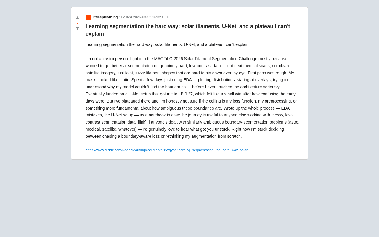
A developer with no background in astronomy entered the MAGFiLO 2026 Solar Filament Segmentation Challenge to push their image segmentation skills on truly difficult data. Their motivation was straightforward: no more practicing on clean medical scans or crisp satellite imagery—instead, they wanted to tackle those faint, blurry filament shapes where even the human eye struggles to identify boundaries.

The core difficulty of this data lies in low contrast and ambiguous boundaries. Solar filaments appear as dark, thread-like structures on the solar disk, with edges that blend imperceptibly into the background. From an astronomical perspective, solar filaments are plasma structures suspended between the solar chromosphere and corona, supported by strong magnetic fields. They appear dark in full-disk Hα (656.3nm) observations because their temperature (~8000K) is far lower than the surrounding corona (~1 million K). When filaments appear at the solar limb, they manifest as bright prominences. Automated detection and segmentation of filaments is critical for solar activity forecasting, as filament eruptions are often associated with coronal mass ejections (CMEs) that can impact Earth's magnetosphere and human space activities.

For the segmentation task, this means the annotations themselves carry inherent ambiguity—when even human experts struggle to precisely delineate boundaries, models will naturally have an even harder time. The MAGFiLO challenge is a benchmark competition at the intersection of solar physics and computer vision, using ground-based or space-based full-disk Hα solar images as input. Since solar filaments vary enormously in morphology—from tiny short filaments to giant filament channels spanning hundreds of thousands of kilometers—and their brightness variations can be confused with chromospheric network structures and flares, this task serves as an extreme testbed for low-contrast semantic segmentation.

EDA First: Understand the Data Before Discussing Architecture

The author's first attempt produced terrible results: "My masks looked like TV static." This is a classic failure mode in low-contrast segmentation—the model cannot find meaningful boundaries in the faint signal, and the predictions are filled with random noise.

To their credit, instead of rushing to tweak the network architecture, they spent several days focused on Exploratory Data Analysis (EDA):

• Plotting pixel intensity distributions to understand the overlap between foreground and background
• Creating overlay visualizations of predicted masks on original images to see what the model was missing
• Staring at the data repeatedly, trying to figure out why the model couldn't find boundaries

EDA in image segmentation tasks goes far beyond simple data visualization. For low-contrast segmentation, key steps include: analyzing the histogram overlap area between foreground/background pixel intensities (which directly reflects the theoretical separability of the task), checking class imbalance ratios (filaments typically occupy only 1-5% of image area), examining annotation consistency (disagreement among multiple annotators on the same sample), and computing statistics on target scale distribution and morphological diversity. When histograms show heavy overlap between foreground and background gray values, it means purely local pixel intensity-based decisions are nearly impossible—the model must rely on contextual information, texture features, or morphological priors to make meaningful predictions.

This step is often overlooked by beginners. When facing difficult data, understanding the statistical properties of your data matters more than blindly stacking model components. When foreground and background intensity distributions heavily overlap, standard segmentation approaches are almost guaranteed to fail—which perfectly explains why early results were pure noise.

The U-Net Approach and Analyzing the 0.27 Score Plateau

After the groundwork laid by EDA, the author ultimately adopted a U-Net architecture and pushed their Leaderboard (LB) score to 0.27. Considering the chaotic early state, this counted as a small victory.

U-Net was originally proposed by Ronneberger et al. in 2015, designed specifically for biomedical image segmentation. Its core innovation lies in skip connections between the symmetric encoder-decoder paths, which concatenate feature maps at different scales from the encoder directly to corresponding decoder layers. This preserves fine spatial information while recovering spatial resolution, enabling the model to leverage both high-level semantic information and low-level spatial details—critical for segmentation tasks requiring precise boundaries.

However, standard U-Net faces several inherent limitations in extremely low-contrast scenarios: its receptive field is constrained by kernel size and network depth, potentially failing to capture global morphological features of filaments; the low-level features passed through skip connections may primarily carry noise rather than effective boundary information in low-contrast images; and U-Net lacks built-in attention mechanisms to selectively enhance feature responses in weak signal regions. Subsequent variants like Attention U-Net, U-Net++, and TransUNet attempt to address these shortcomings from different angles. The 0.27 score confirms that standard U-Net hits a clear ceiling on this type of extremely ambiguous data.

Where Does the Bottleneck Actually Come From?

The author honestly listed three possible "culprits" but couldn't determine which one was dominant:

1. Poorly designed loss function: Common cross-entropy or Dice Loss have limited ability to handle ambiguous boundaries
2. Insufficient preprocessing: Low-contrast data may require more aggressive contrast enhancement or normalization strategies
3. Theoretical ceiling from annotation ambiguity: These boundaries are inherently fuzzy, imposing an insurmountable performance ceiling

The third point is particularly thought-provoking. Quantifying annotation ambiguity corresponds to the concept of Bayes error rate in machine learning theory. When multiple experts show significant disagreement on the boundary annotations of the same filament, this inter-annotator variability defines the irreducible error lower bound of the task. In practice, you can estimate this ceiling by having multiple annotators independently label the same data and computing inter-annotator Dice coefficients—if annotator agreement is only 0.6, then any model exceeding this level may be overfitting to a particular annotator's preferences. In recent years, probabilistic segmentation methods (such as Probabilistic U-Net) and distribution-based prediction approaches attempt to directly model this uncertainty, outputting multiple plausible segmentation hypotheses rather than a single deterministic prediction—especially valuable in domains where annotations themselves are contested.

When the ground truth itself carries subjectivity and uncertainty, the model's performance ceiling may not stem from technical deficiencies but from the inherent ambiguity of the task itself. At that point, even infinite tuning won't break through.

Two Paths to Breaking the Plateau: Boundary-Aware Loss and Data Augmentation Redesign

The author is currently at a typical crossroads, debating between two improvement directions:

Direction One: Introducing Boundary-Aware Loss Functions

To address the fuzzy boundary problem, one can introduce loss functions that specifically reinforce boundary regions, such as:

• Boundary Loss: Proposed by Kervadec et al. in 2019, it reformulates segmentation as predicting a distance field from pixels to true boundaries, explicitly modeling errors near boundaries by directly incorporating boundary distance metrics into the loss
• Focal Loss: Uses the modulating factor (1-p)^γ to down-weight easily classified samples, making the model focus on difficult boundary pixels and transitional zones
• Dice + BCE combination: Balances region overlap with pixel-level accuracy

In segmentation tasks with ambiguous boundaries, the choice of loss function directly impacts how the model learns about uncertain regions. Standard Binary Cross-Entropy treats each pixel as an independent binary classification problem, penalizing misclassifications in boundary and interior regions equally, which can cause the model to output large areas of intermediate probability values at fuzzy boundaries. Dice Loss is based on region overlap metrics, more friendly to small targets but with unstable gradients at boundaries. In practice, weighted multi-loss combinations (e.g., 0.5×Dice + 0.5×BCE + 0.1×Boundary) with dynamic adjustment across training phases often perform best.

The idea behind these approaches is to make the model "try harder" to focus on those difficult-to-determine transitional zones.

Direction Two: Redesigning Data Augmentation from Scratch

The other path is to redesign the data augmentation strategy entirely. For low-contrast data, simple flips and rotations may be far from sufficient. What's needed might include:

• Targeted contrast/brightness perturbations
• Elastic deformations to simulate the variable morphology of filaments
• Noise injection that matches astronomical imaging characteristics

Data augmentation for astronomical low-contrast images needs to consider physical plausibility. CLAHE (Contrast Limited Adaptive Histogram Equalization) can serve as a preprocessing step to enhance local contrast, but its parameters (clipLimit and tileGridSize) need careful tuning to avoid over-amplifying noise. Gamma transformations can simulate different exposure conditions. More specialized strategies include: simulating solar limb darkening through radial brightness attenuation, physically-motivated noise injection based on Poisson noise models (solar observation is fundamentally a photon counting process), and thin-plate spline (TPS) elastic deformations tailored to the serpentine morphology of filaments. It's worth noting that Mixup and CutMix-style augmentations should be used cautiously, as the filamentary morphology can easily lose semantic coherence during mixing. Additionally, Test-Time Augmentation (TTA)—averaging predictions across multiple augmented versions—may provide extra gains at inference time.

General Lessons for Low-Contrast Segmentation Tasks

Although this case focuses on solar filaments, the lessons are applicable to all low-contrast, boundary-ambiguous segmentation tasks—whether in astronomy, medical imaging, or satellite remote sensing, the fundamental challenges are the same.

Key takeaways:

• Never skip EDA: When facing difficult data, understanding the data distribution before touching architecture saves many wrong turns
• Be aware of the ambiguity ceiling in the data itself: Performance bottlenecks aren't necessarily technical problems—they may reflect inherent annotation uncertainty. Estimate the theoretical performance ceiling by computing inter-annotator agreement
• U-Net is a starting point, not an endpoint: On extreme data, loss function design and data augmentation are often more impactful than switching to a larger model. Consider attention mechanisms (Attention U-Net), multi-scale feature fusion (U-Net++), or Vision Transformers (TransUNet) as next-step architectural upgrades
• The value of physical priors: For specialized domains like astronomy or medicine, encoding domain knowledge (such as solar limb darkening or magnetic topology constraints of filaments) as model inductive biases or data augmentation strategies is often more effective than generic approaches

The author concluded by reaching out to the community: if you've tackled similar fuzzy boundary segmentation challenges, what helped you break through the plateau? This is precisely the value of open source and community collaboration—truly difficult problems often require cross-disciplinary experience and cross-pollination of ideas to find answers.