Visualizing Neural Network Learning: How ReLU Fits Arbitrary Functions
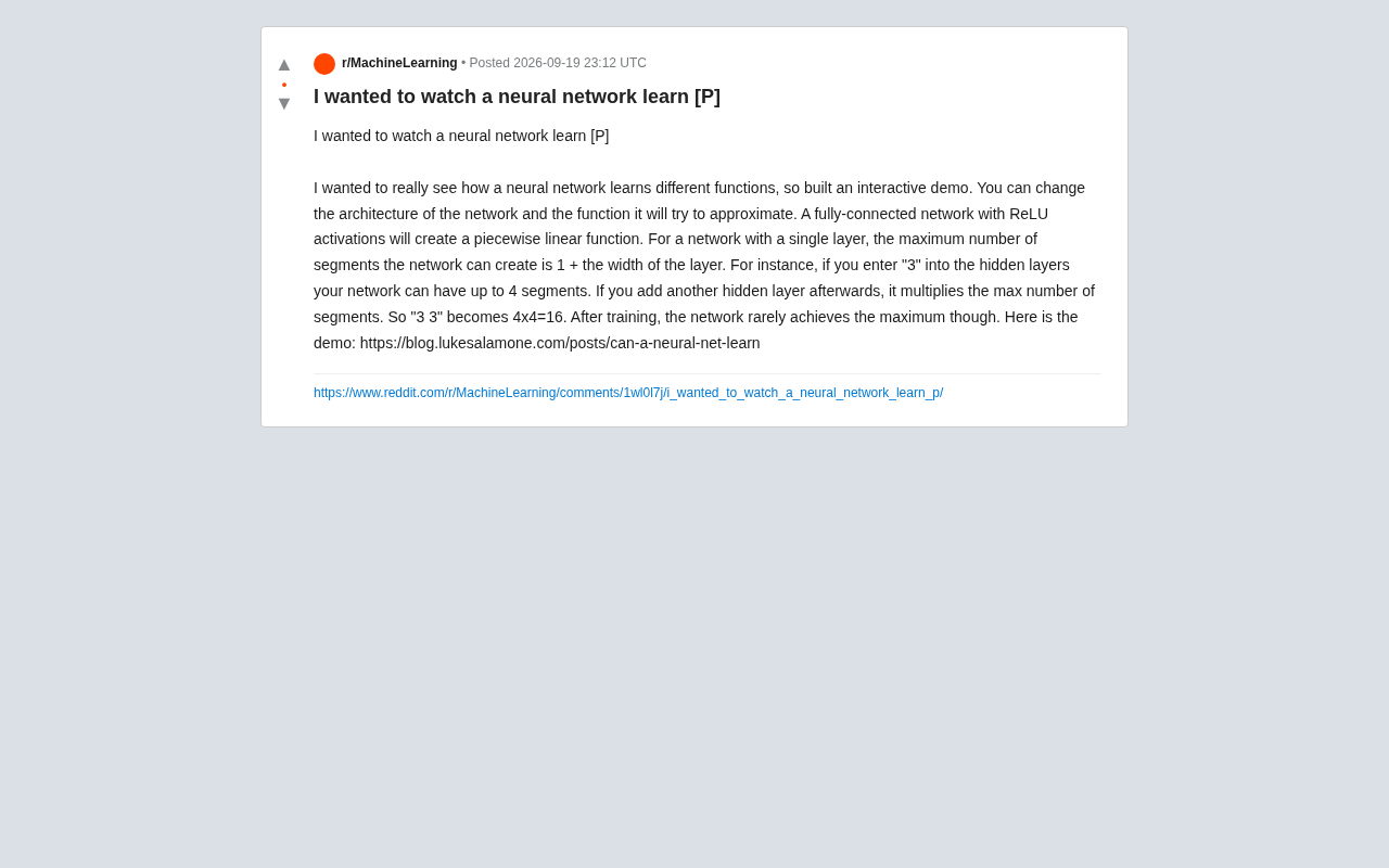
Interactive demo reveals how ReLU neural networks use piecewise linear functions to approximate targets, with depth driving exponential capacity growth.
Developer Luke Salamone built a browser-based interactive demo that lets users directly observe neural network training. The key insight: fully connected networks with ReLU activations are fundamentally approximating target curves with piecewise linear functions. A single hidden layer produces at most "1 + width" segments, while adding layers multiplies segment counts — an exponential growth that geometrically explains why depth is more efficient than width. The demo also reveals that networks rarely use their theoretical maximum segment count after training, reflecting gradient descent's implicit bias toward simpler, lower-degree-of-freedom solutions. For learners building intuition about deep learning, this kind of visualization tool far outweighs static formula-based explanations.
When Neural Network Learning Becomes Visible
For many people, neural networks remain a black box: data goes in, results come out, and the weight adjustments in between happen like magic. Developer Luke Salamone wanted to demystify this process, so he built an interactive demo that lets users actually see how a neural network gradually learns to approximate a target function.
The core idea is straightforward: rather than reading through equations, you watch the network adjust its shape step by step during training until it fits the target curve. Users can freely modify the network's architecture and the target function it needs to fit — all in the browser — and observe the training dynamics in real time. The demo is available at blog.lukesalamone.com.
![reddit source: I wanted to watch a neural network learn [P]](/media/screenshots/source/28906_0.png)
The Geometric Nature of ReLU Networks: Piecewise Linear Functions
This demo reveals a profound but often overlooked fact — fully connected networks using ReLU activations fundamentally construct a piecewise linear function. In other words, no matter how smooth the target curve is, a ReLU network approximates it with a series of straight line segments. The more segments, the smoother the approximation.
This is tremendously helpful for understanding the capability boundaries of deep learning. ReLU's nonlinearity comes from its "break" at zero: each neuron can contribute one breakpoint. Stack enough neurons together, and you get a complex shape assembled from many line segments. In theory, given enough segments, any continuous function can be approximated to arbitrary precision — this is the intuitive embodiment of the Universal Approximation Theorem.
How Segment Count Is Calculated
The author provides a clear quantitative rule for estimating how many line segments a network can produce:
- Single-layer network: The maximum number of segments equals
1 + layer width. For example, entering "3" for the hidden layer means the network can produce at most 4 segments. - Multi-layer network: Segment counts across layers multiply together. For example, a "3 3" architecture (two hidden layers of width 3) yields a maximum of 4 × 4 = 16 segments.
This multiplicative relationship intuitively explains why depth matters so much. Compared to simply increasing the width of a single layer (which grows segment count linearly), adding depth causes expressive capacity to grow exponentially. This is a geometric explanation for why deeper networks often outperform shallower networks with the same parameter count.
ReLU (Rectified Linear Unit) is the most widely used activation function in modern deep learning, defined simply as f(x) = max(0, x) — output is zero for negative inputs and passes positive inputs through unchanged. This "zero out the negatives" break is what gives each neuron a boundary point in input space. To the left of that point, the neuron's output is always zero (a "dead" state); to the right, output increases linearly with input. Combining large numbers of such neurons — each with its breakpoint at a different location — produces a piecewise linear function assembled from many segments. Compared to earlier activations like Sigmoid or Tanh, ReLU's key advantage is that its gradient is always 1 on the positive side, effectively mitigating the vanishing gradient problem in deep networks, while being computationally cheap. Understanding this geometric interpretation of ReLU — that each neuron contributes one potential breakpoint — is the foundational intuition for grasping a network's expressive capacity.
The Universal Approximation Theorem is one of the cornerstone results in deep learning theory. It states that a feedforward neural network with at least one hidden layer, sufficiently many neurons, and a nonlinear activation function can approximate any continuous function defined on a compact set to arbitrary precision. This mathematically guarantees that neural networks can, in principle, learn anything. However, the theorem only proves existence — that some set of weights achieves the approximation — without telling us whether gradient descent can find those weights, or how many neurons or training samples are needed. The theorem is therefore more of a theoretical "upper bound on capability" than a practical guarantee. The segment-count rule provides a concrete, quantifiable geometric interpretation of this abstract theorem: as depth increases, the number of available breakpoints grows exponentially, and approximation capacity rises sharply in turn.
The Gap Between Theoretical Capacity and Actual Training
The author highlights an intriguing observation: after training, networks rarely reach their theoretical maximum segment count.
This touches on a fundamental gap between theoretical capacity and practical performance in deep learning. A "3 3" architecture can theoretically produce 16 segments, but after gradient descent training, the number of effective segments is often far lower. The reasons include:
- Gradient descent seeks solutions that minimize loss — it doesn't deliberately use up all available expressive capacity.
- Many neurons' breakpoints may fall outside the data range, or multiple breakpoints may collapse and coincide.
- The complexity of the target function determines how many segments are actually needed; simple functions don't require the full capacity.
This reminds us that a network's theoretical capacity (what it can represent) and the solution it actually learns (what it represents after training) are two distinct things. Part of the reason over-parameterized networks tend not to overfit is precisely that the training process gravitates toward "simpler" solutions with fewer effective degrees of freedom.
Over-parameterization refers to a model having far more parameters than the minimum required to fit the training data. Classical statistics predicts that over-parameterization necessarily leads to overfitting — but deep learning practice has repeatedly shown the opposite: over-parameterized neural networks often generalize better. This phenomenon appears in what's known as the "double descent" curve, and has sparked extensive theoretical research in recent years. Among the many solutions that could perfectly fit the training set, gradient descent naturally favors "flatter" and "simpler" ones — an implicit regularization effect believed to be closely tied to generalization performance. The observation in this demo — that the number of segments after training is far below the theoretical maximum — is a geometric manifestation of this implicit bias: the network doesn't use all its breakpoints, instead converging to a simpler solution with fewer degrees of freedom, which aligns with the behavior of well-generalizing networks.
Why Visualization Tools Like This Matter
For learners, interactive demos like this offer far greater pedagogical value than static textbooks. By hands-on tweaking of architecture and watching the fitting process unfold, several abstract concepts become concrete:
- How architecture affects expressive power: The different effects of going wider vs. going deeper become immediately obvious.
- The geometric meaning of activation functions: Why ReLU produces piecewise lines rather than smooth curves.
- Training dynamics: The network doesn't jump to a solution — it gradually adjusts the slope and position of each line segment.
This kind of "visible" learning bridges the gap that equation-based derivations struggle to fill intuitively. It continues the tradition of tools like TensorFlow Playground — turning the internal mechanics of deep learning from a black box into an explorable sandbox.
Summary
This interactive demo, built by a community developer, explains a core principle in the most direct way possible: a ReLU fully connected network approximates its target using piecewise linear functions. The rules — that segment count grows linearly with width and exponentially with depth, and that actual training rarely exhausts theoretical capacity — are all made viscerally clear through visualization. For anyone who wants to genuinely understand the internal mechanics of neural networks rather than just use them as a black box, spending time with this demo will deliver more insight than reading ten pages of textbook.
Related articles

A Meta Senior Engineer's Deep Dive into AI-Assisted Programming: Is Hand-Written Code Dying?
A Meta L7 engineer shares real-world AI coding insights: why hand-written code is fading, how to review AI output, Codex vs Claude Code, and career advice for the AI era.

Qwen Image 2.1 Open Source Release Imminent: VRAM Requirements Dominate Community Discussion
Qwen Image 2.1 open-source release is imminent. Community discussion centers on VRAM requirements — can it run on mainstream 12–16GB consumer GPUs?

PlanetScale Launches Tin: A Full-Text Search Solution Built for Postgres
PlanetScale launches Tin, a full-text search tool built for PostgreSQL that aims to eliminate the need for separate search engines like Elasticsearch.