A Complete Guide to RAG Evaluation Metrics: Retrieval, Generation, and Operations

RAG system evaluation often drowns people in a sea of metrics: libraries expose dozens of them, dashboards display them side by side in the same font size, and every one looks equally important. But in practice, only a handful actually drive decisions. Understanding what each metric answers is more valuable than tracking all of them.

RAG metrics fall into three categories: retrieval metrics determine whether the system recalled the right chunks; generation metrics determine whether the LLM made good use of that content; and operational metrics determine whether you can afford to run the whole thing.

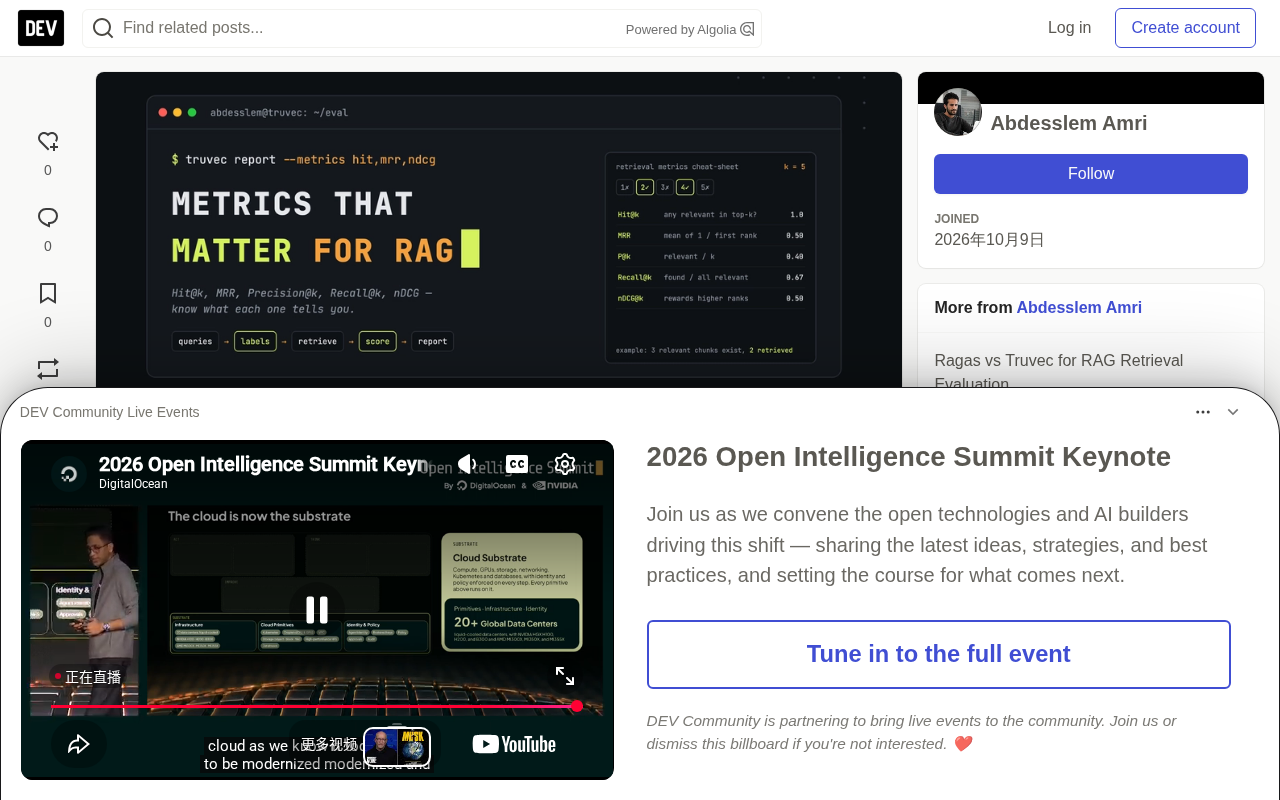
Retrieval Metrics: Did It Find the Right Things?

Retrieval metrics compare the chunks returned by the retriever against a known "golden dataset" that contains the answers. All calculations are based on the Top-K results for each question, then averaged across all questions.

Suppose the golden dataset labels the expected chunks for a given question, and the retriever is configured to return Top-5 results. Using this concrete example, we can compute each metric one by one.

Hit rate@k: Did it find anything useful?

If at least one expected chunk appears in the Top-K, the metric is 1; otherwise 0. Averaged across all questions, it represents the proportion of questions for which the LLM received at least part of the information it needed.

In the example, #14 appears in the Top-5, so hit rate = 1.

This is the easiest metric to interpret, but it ignores ordering and completeness—finding one is indistinguishable from finding all under this metric.

Recall@k: How much of the answer-relevant content was found?

The number of expected chunks retrieved divided by the total number of expected chunks.

In the example, only 1 of 2 expected chunks was found, so recall@5 = 0.5.

Recall@k matters especially when answers are spread across multiple chunks. Missing some chunks means the LLM only has half the facts available—that's how incomplete answers happen.

Precision@k: How much of what was retrieved is actually useful?

The number of expected chunks retrieved divided by k.

In the example, precision@5 = 1/5 = 0.2.

This metric needs to be interpreted carefully. When there is only one expected chunk and k=5, the theoretical ceiling for precision is just 20%. It's good for comparing two configurations, not as an absolute score. It only deserves more attention when context is expensive or irrelevant chunks clearly distract the LLM.

MRR: Where does the first correct chunk rank?

Mean Reciprocal Rank: the reciprocal of the rank of the first expected chunk, or 0 if not found.

In the example, the first expected chunk ranks at position 2, so MRR = 1/2 = 0.5.

This is the metric most worth prioritizing. LLMs pay more attention to earlier passages, and many systems only use the Top-1 to Top-3 chunks. Two models with the same hit rate—one placing the answer first and the other fifth—are not equivalent.

nDCG@k: How good is the overall ranking quality?

Normalized Discounted Cumulative Gain scores each expected chunk that was found, applies a larger discount for lower ranks (logarithmic discount), then divides by the score of a perfect ranking. Values range from 0 to 1.

In the example, 1 of 2 expected chunks ranks at position 2. Assuming binary relevance, DCG = 1/log₂(3) ≈ 0.63; an ideal ranking would place both chunks at rank 1 and rank 2, giving ideal DCG = 1 + 0.63 = 1.63, so nDCG@5 ≈ 0.39.

nDCG@k attempts to answer two questions with a single number: "were all the needed chunks found" and "are they ranked near the top." It is the standard metric for retrieval benchmarks (MTEB's retrieval task reports nDCG@10), and a good single number to report when answers frequently span multiple chunks.

The core idea of Discounted Cumulative Gain (DCG) is that the higher a relevant chunk appears in the ranking, the more it contributes to overall retrieval quality. In calculation, each relevant chunk is assigned a discount factor based on its rank position (typically 1/log₂(rank+1)), with lower ranks discounted more heavily, and then all discounted scores are summed. Ideal DCG is the maximum score achievable if all relevant chunks were perfectly ranked at the top. nDCG is DCG divided by ideal DCG, normalizing the score to between 0 and 1 so results can be compared across questions with different numbers of relevant chunks. nDCG also supports graded relevance—not just a binary "relevant/irrelevant" judgment, but assigning each chunk a relevance level like 0, 1, 2, or 3 (e.g., "fully answers," "partially relevant," "merely mentions"), which is especially useful in question-answering tasks. For this reason, mainstream retrieval benchmarks like MTEB universally report nDCG@10 as their preferred metric.

Diagnostic Retrieval Metrics: Why That Score?

Beyond the core metrics, three patterns help explain why retrieval performs the way it does.

Hit rate by cutoff (hit rate@1, @2 ... @k) forms a curve. If the curve starts low but keeps climbing, the model found the right region but didn't rank the best chunk near the top—increasing Top-K or adding a reranker usually helps.

The rank distribution of the first relevant chunk separates "near miss" (ranking 4th or 5th in a Top-5 scenario) from "complete failure."

Score gap is the similarity of the best expected chunk minus the similarity of the best incorrect chunk (the highest distractor). A large positive gap means stable ranking; a gap near zero means the correct chunk and a similar chunk are nearly tied, and a slight rephrasing could flip the result. Near-duplicate documents and heavily templated chunks are common causes.

Generation Metrics: Is the Answer Well Written?

Once retrieval is solid, evaluation moves to the answers themselves. These metrics typically use an LLM as a judge, computed via libraries like Ragas:

• Faithfulness/Groundedness: Are the claims in the answer supported by the retrieved context?
• Answer relevance: Does the answer address the question asked?
• Answer correctness: Does the answer agree with the reference answer?
• Context precision and context recall (LLM-judged versions): Use a judge model to assess relevance rather than relying on known chunk IDs.

Judge models themselves have errors and biases, and swapping the judge model or prompt shifts scores. Moreover, a low faithfulness score doesn't tell you whether the LLM ignored good context or never received it in the first place—only retrieval metrics based on known chunk IDs can answer that.

LLM-as-a-judge is currently the dominant paradigm for evaluating generation quality. The typical workflow is: given the question, the retrieved context, and the model-generated answer, a capable LLM (at the GPT-4 level) judges faithfulness, relevance, or correctness item by item according to a predefined rubric, outputting a score or rationale. The advantages are no manual annotation required, strong scalability, and the ability to handle semantic-level evaluation of open-ended answers; frameworks like Ragas implement metrics such as faithfulness and answer relevance on this basis. But its limitations are obvious too: biases in the judge model itself (such as favoring longer answers or preferring certain phrasing styles) systematically affect scores; scores are not directly comparable across different judge models or prompt versions; and when the judging criteria are vague, the same answer may receive different verdicts across runs. Engineering practice therefore suggests fixing the judge model and prompt version, and supplementing with a small amount of human calibration in critical scenarios.

Operational Metrics: Can You Afford to Run It?

Quality is only half the decision. Every retrieval configuration also needs to be measured on operational cost:

• Indexing cost: The one-time cost of embedding the full corpus, plus the recurring cost each time you rebuild the index or switch models.
• Cost per thousand queries: The cost of embedding user questions at actual traffic volume.
• Query latency: The time to convert a question into a vector plus vector search time (p50 and p95).
• Vector storage: Number of chunks × dimensions × 4 bytes (float32 vectors). A 3072-dimensional model needs twice the storage of a 1536-dimensional one.

Embeddings typically account for only a small fraction of RAG system costs (compared to LLM calls), but they can't be ignored at scale: large corpora, frequent index rebuilds, and high query volume all amplify their impact.

Estimating vector storage capacity is the most commonly underestimated part of the planning phase. Vectors stored as float32 take 4 bytes per dimension, so a 1536-dimensional chunk vector occupies 1536 × 4 ≈ 6KB, and one million chunks require about 6GB of pure vector storage; with a 3072-dimensional model, the same count needs about 12GB. And that's just the raw vectors—real deployments often also need to store metadata, raw text, and vector index structures (like HNSW graphs or IVF inverted lists), which can add another 30%–50% or more in space overhead. Dimension choice is therefore a cost-versus-quality tradeoff: higher dimensions may bring better semantic discrimination, but storage and search costs rise proportionally, and search latency grows with dimension. Before settling on an embedding model, running a storage and latency estimate with your expected corpus size often prevents forced rework after launch.

Tooling in Practice: Truvec's Metric Coverage

Truvec focuses on the retrieval and operations layers. It evaluates embedding models and chunking strategies on your own documents using a golden dataset that you review and lock, so scores are deterministic and comparable over time. It does not evaluate generated answers.

For every model in each evaluation and comparison, Truvec reports the following:

Quality metrics (at your chosen Top-K, 1 to 50, default 5): Hit rate, Recall@k, Precision@k, MRR, nDCG@k, F1@k.

Diagnostics: Hit rate by cutoff curve, first relevant chunk rank distribution (including misses), score gap, average relevant score and highest distractor score.

Cost, speed, and storage: Indexing cost and cost per thousand queries (based on actual billed tokens and the model's per-million-token price), current run billing, query embedding latency, vector search p50/p95, vector storage and dimensions.

Per-question analysis: Retrieval Inspector shows the chunks retrieved for each question by rank, labeled as Ground truth or Distractor with similarity scores, and also displays chunks that were "expected but not retrieved." Filter by Misses to see what each model missed. In comparison mode, models are sorted by MRR then by recall, and the PDF report includes head-to-head analysis and a matrix showing each question's first relevant chunk rank under each model.

Which Metrics Should You Watch?

The choice of metrics depends on your specific configuration. If answers typically fall in a single chunk, prioritize MRR and Hit rate; if answers span multiple chunks, Recall@k and nDCG@k matter more. Precision@k only makes sense when the context window is tight or distractors are obvious. Introduce generation metrics after retrieval is stable, to avoid mistaking retrieval problems for LLM problems. Operational metrics should be weighed flexibly based on corpus size and query volume.

One-line Summary

RAG evaluation metrics fall into retrieval, generation, and operations categories, with MRR and nDCG as the core, chosen by scenario.

Paragraph Summary

The article systematically divides RAG system evaluation metrics into three categories: retrieval, generation, and operations. Retrieval metrics (Hit rate, Recall@k, Precision@k, MRR, nDCG@k) measure recall quality against a golden dataset, with MRR most worth prioritizing since LLMs pay more attention to earlier passages; nDCG@k measures both completeness and ranking quality and is the standard metric for retrieval benchmarks. Generation metrics (faithfulness, answer relevance, correctness, etc.) rely on LLM judging but suffer from judge bias and cannot distinguish whether the LLM ignored the context or never received it. Operational metrics cover indexing cost, cost per thousand queries, latency, and vector storage. The article also introduces diagnostic metrics like hit rate curves, rank distributions, and score gaps, and uses the Truvec tool as an example to illustrate metric coverage in the retrieval and operations layers. The core recommendation is to choose metrics by configuration: use MRR for single-chunk answers, Recall and nDCG for cross-chunk answers, and introduce generation metrics only after retrieval is stable.