Analog In-Memory Computing Fault Localization: Sparse Recovery Decoder Needs Only 4-12 Reads

New preprint uses sparse recovery decoder to cut analog crossbar fault localization reads from 256 to 4-12, proactively disclosing several pre-registered failed conclusions.
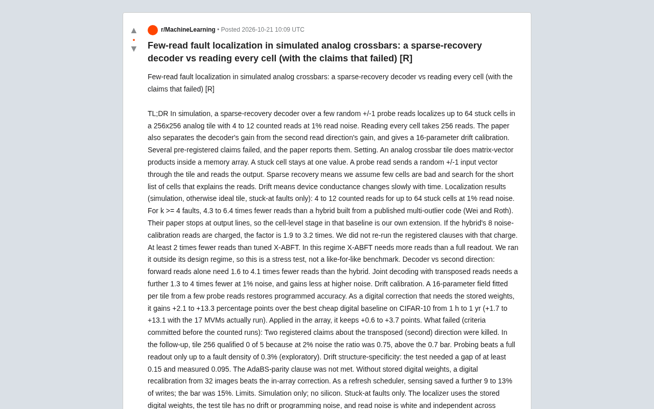
A preprint proposes using a sparse recovery decoder to localize stuck-at faults in analog crossbars, reducing reads for a 256×256 tile from 256 (full cell-by-cell readout) to 4-12, handling up to 64 faulty cells. The paper reports decoder gain and transposed-direction read gain separately: forward reads require 1.6-4.1 times fewer than the hybrid baseline, and joint decoding requires 1.3-4 times fewer. It also proposes a 16-parameter drift calibration field, achieving 2.1-13.3 percentage points higher than cheap digital baselines on CIFAR-10. The authors proactively disclose several pre-registered conclusions that did not hold up and list limitations including pure simulation, white noise assumptions, and overly tight confidence intervals, openly soliciting criticism on the baseline and noise model.
In analog crossbars, the traditional way to locate bad cells is cell-by-cell readout—a 256×256 tile requires 256 reads. A new preprint proposes using a sparse recovery decoder to cut the number of reads to 4 to 12 in simulation, while the authors proactively disclose several pre-registered conclusions that did not hold up.
Background: Why "reading less" matters
Analog in-memory computing performs matrix-vector multiplication inside the memory array, eliminating the data movement overhead. The cost is imperfect devices: stuck-at faults get pinned to a fixed value, and conductance drifts over time. To ensure trustworthy computation results, you need to know which cells are faulty.
The most direct localization method is cell-by-cell readout, requiring 256 reads for a 256×256 tile. Each read means one probe input and one output sample, burdening both test time and peripheral circuitry. The core question of this paper is: can we locate faulty cells using far fewer than 256 random ±1 probe reads?
The idea borrows from compressed sensing: since faults are sparse (only a few), there's no need to read all cells. Instead, design a small number of random probes and reverse-solve the short list of faulty cells from the outputs.
Compressed sensing and sparse recovery: The core idea of compressed sensing is that if a signal is sparse in some basis (i.e., only a few non-zero entries), it can be recovered from linear observations far fewer than the Nyquist sampling count, typically by solving a least-squares problem with L1-norm regularization (such as Lasso), whose solution tends to be sparse. This paper treats the list of faulty cells as a sparse signal, random ±1 probe reads as the observation matrix, and the decoder searches for the shortest fault list that explains the observations. Note that recovery guarantees in compressed sensing typically depend on the restricted isometry property (RIP) of the observation matrix and on noise levels; when fault density rises or noise is not independent white noise, recovery performance degrades significantly—this is the theoretical root of the applicability boundary (fault density below ~0.3%) noted by the authors.
Core method: sparse recovery decoder
The authors build an idealized tile in simulation, injecting only stuck-at faults, with read noise set to 1% white noise independent across directions. The probe read process is: input a random ±1 vector to the tile, read the output vector. Multiple such reads form an observation matrix, and the decoder assumes faulty cells are sparse, searching for the shortest fault list that explains these observations.
Result: with up to 64 stuck-at cells, the read count is 4 to 12. As a comparison, a hybrid baseline constructed from published multiple-outlier coding (Wei and Roth) requires 4.3 to 6.4 times more reads at k≥4 faults—though the baseline only goes to the output-line level, and the cell-level stage is the authors' own extension; if the hybrid baseline's 8 noise-calibration reads are also counted, the ratio drops to 1.9 to 3.2 times. The authors also note that they did not re-run the registered clauses using this accounting method.
Another baseline is a tuned X-ABFT, which the paper reports requires at least 2 times fewer reads. But the authors honestly point out that X-ABFT in this scenario requires more reads than full readout, making it a stress test outside its design scope rather than an equivalent benchmark.
X-ABFT and multiple-outlier coding: X-ABFT is a class of online fault-tolerance techniques for matrix operations. Its basic approach is to apply checksums to the rows/columns of the input matrix and detect and localize computation faults by comparing output checksums against expected values—a lightweight checksum-based scheme. Multiple-outlier coding (Wei and Roth), on the other hand, designs coding matrices so that a small number of outlier errors can be identified and corrected during decoding, originally used for fault recovery in distributed storage. The hybrid baseline cited in this paper transplants such coding ideas to cell-level localization in crossbars, but the original scheme only goes to the output-line level, and the cell-level stage is the authors' own extension. X-ABFT requires even more reads than full readout in this scenario because its checksum granularity does not match the array fault model—making it a stress test rather than an equivalent benchmark.
Separating decoder gain from second-direction gain
The paper deliberately separates two sources of gain: the gain from the decoder itself, and the gain from transposed-direction reads. With forward reads only, it requires 1.6 to 4.1 times fewer reads than the hybrid baseline; joint decoding plus transposed reads requires 1.3 to 4 times fewer at 1% noise. As noise increases, the gain from the second direction diminishes.
This separation is valuable because it answers "what exactly is doing the work." Many compressed-sensing-style works report multiple gains mixed together, leaving readers unable to tell whether the benefit comes from the algorithm or from additional hardware accesses.
However, the authors explicitly state that they have not proven that two directions necessarily require fewer reads than one, and transposed reads also assume bidirectional peripheral circuitry whose cost has not been validated.
Drift calibration: 16-parameter field
Beyond fault localization, the paper also presents a drift calibration scheme: each tile fits a 16-parameter field using a small number of probe reads, restoring programming accuracy.
As a digital correction requiring stored weights, on CIFAR-10, from 1 hour to 1 year, it is 2.1 to 13.3 percentage points higher than the best cheap digital baseline (1.7 to 13.1 counting the 17 MVMs actually run). Applied directly in-array, it retains a gain of 0.6 to 3.7 points. These numbers show: digital correction yields greater benefit but requires reading out weights; in-array correction yields smaller benefit but avoids the data movement.
Conductance drift and programming accuracy: In analog in-memory computing, the conductance of resistive devices (such as RRAM/PCM) drifts over time, typically manifesting as power-law relaxation (conductance drift), where conductance slowly decays over time as (G(t)=G_0 (t/t_0)^{-\nu}), with the drift rate correlated with the programmed conductance level. This causes stored weight values to deviate from programming targets, degrading inference accuracy. Digital correction first reads out weights and recomputes compensation in the digital domain; in-array correction adjusts in place by applying additional programming/read pulses. The 16-parameter field is a low-dimensional parametric model of drift behavior, fitting these parameters with a small number of probe reads to restore programming accuracy without cell-by-cell readout. Its benefit is limited by whether the model can capture the spatiotemporal correlations of real drift.
Failed claims: what the authors proactively disclose
What is relatively rare about this preprint is that the authors list conclusions that were pre-registered but did not hold up.
Two registered clauses about the transposed (second) direction were rejected. In follow-up experiments, 0 of 5 for tile 256 passed, because the ratio at 2% noise was 0.75, above the 0.7 threshold. Exploratory analysis shows that probe reads outperform full readout only when fault density is below 0.3%.
The drift structure-specificity test required a gap of at least 0.15; the measured value was 0.095, falling short. The AdaBS equivalence clause was not met.
Without stored digital weights, digital recalibration using 32 images actually outperformed in-array correction. As a refresh scheduler, sensing saved only an additional 9 to 13% of writes, against a threshold of 15%.
These failed items are more informative to readers than the successes: they delineate the applicability boundaries of the method.
Limitations and points for debate
The paper's limitations are clearly listed: pure simulation, no silicon validation; only stuck-at faults considered; the localizer uses stored digital weights; test tiles have no drift or programming noise; read noise is white and direction-independent.
Statistically, the 240 instances per cell are clustered but treated as independent, making confidence intervals too tight. The registration criteria are in the authors' own repository, not a third-party registration platform. Absolute accuracy did not pass CrossSim validation, with differences up to 5.66 points against a threshold of 0.5.
The authors openly solicit criticism at the end, specifically calling out the baseline and noise model. From a reviewer's perspective, the most pressing questions are: does the white noise assumption hold in real arrays? Will the peripheral cost of transposed reads offset the read-count benefit? And when fault density exceeds 0.3%, does the sparse recovery assumption still hold?
Sources: Reddit r/ discussion thread and the preprint (Zenodo DOI: 10.5281/zenodo.23472381), code at GitHub prateek1656/NeuroFault.
CrossSim validation and clustered confidence intervals: CrossSim is an open-source analog in-memory computing simulator developed by Sandia National Laboratories, supporting multiple device models, noise, and drift, and is often used as a reference simulation platform for crossbar algorithm research. This paper's absolute accuracy did not pass CrossSim validation (differences up to 5.66 points), indicating a gap between its idealized simulation and more realistic device models, which may affect the transferability of conclusions. On the other hand, the paper treats 240 instances per cell as independent samples when computing confidence intervals, but these instances come from clustered structures within the same tile and exhibit intra-group correlation, leading to underestimated standard errors and overly tight confidence intervals; a more robust approach would be to use cluster-robust standard errors or stratified bootstrapping.
One-line Summary
A new preprint uses a sparse recovery decoder to cut analog crossbar fault localization reads from 256 to 4-12, and proactively discloses several pre-registered failed conclusions.
Paragraph Summary
A preprint proposes using a sparse recovery decoder to localize stuck-at faults in analog crossbars, reducing reads for a 256×256 tile from 256 (full cell-by-cell readout) to 4-12, handling up to 64 faulty cells. The paper reports decoder gain and transposed-direction read gain separately: forward reads require 1.6-4.1 times fewer than the hybrid baseline, and joint decoding requires 1.3-4 times fewer. It also proposes a 16-parameter drift calibration field, achieving 2.1-13.3 percentage points higher than cheap digital baselines on CIFAR-10. The authors proactively disclose several pre-registered conclusions that did not hold up and list limitations including pure simulation, white noise assumptions, and overly tight confidence intervals, openly soliciting criticism on the baseline and noise model.
Related articles

Grok Bot vs ChatGPT Agent: Which AI Agent Is More Powerful?
How does Grok Bot differ from ChatGPT Agent? This comparison examines how they work: Grok Bot has a cloud computer and runs persistently inside tools to execute multi-step tasks automatically; ChatGPT Agent operates web pages in a browser and is more mature at general tasks. Includes selection advice.

Walmart Agent Gateway: AI Shops for You Automatically—Why Is Amazon Going the Opposite Way?
Walmart's Agent Gateway lets ChatGPT, Gemini and other AI assistants access its product catalog to search, compare and add to cart, with spending limits and per-purchase approval. Amazon blocks external AI agents—two retail giants, opposite paths. Currently US-only, India may follow.

Walmart Opens Shopping to AI Agents: ChatGPT and Gemini Can Place Orders
Walmart launches Agent Profiles, allowing AI agents like ChatGPT, Gemini, and Meta Muse to shop for users with spending limits, per-transaction approval, and isolated orders—no Walmart Plus required. This article analyzes how it works and its industry impact, in stark contrast to Amazon's blocking of AI agents.