Bayesian Inference in Practice: A Complete Guide from Theory to Python Implementation

Introduction: Why Bayesian Inference Deserves a Fresh Look

Among the many theoretical tools in machine learning, Bayesian Inference has always occupied a central position. It is not only an important branch of probability theory but also a key framework for understanding uncertainty in modern machine learning models.

Bayesian inference is a statistical inference method proposed by 18th-century British mathematician Thomas Bayes. Unlike frequentist statistics, which views probability as the long-term frequency of event occurrence, the Bayesian school interprets probability as a subjective measure of belief about uncertainty. This difference manifests in parameter estimation: frequentists regard parameters as fixed but unknown values, while Bayesians treat parameters themselves as random variables that can be described by probability distributions. This philosophical difference makes Bayesian methods naturally suited for small sample problems and online learning scenarios—whenever new data arrives, we simply update the posterior distribution without retraining the entire model. In recent years, with the maturation of computational methods like variational inference and Markov chain Monte Carlo, Bayesian methods have found widespread application in deep learning, particularly in uncertainty quantification and active learning.

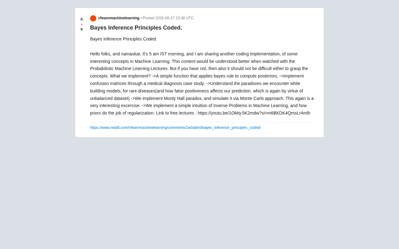
Recently, a developer shared a code implementation of Bayesian inference principles on Reddit, covering multiple practical topics from the basics of Bayes' theorem to Monte Carlo simulation. The value of this content lies not in stopping at theoretical derivations but in making abstract concepts concrete through runnable code. The author suggests watching it alongside Probabilistic Machine Learning Lectures for best results, but even without prior background, readers can gradually understand these core concepts through the code.

Five Key Code Implementations of Bayesian Inference

Bayes' Theorem and Posterior Probability Calculation

The starting point of the entire implementation is a simple yet foundational function—applying Bayes' rule to calculate posterior probability. The mathematical expression of Bayes' theorem is:

P(A|B) = P(B|A) × P(A) / P(B)

Behind this seemingly simple formula lies the profound idea of "updating beliefs with new evidence." In the code implementation, we can intuitively see how prior probability transforms into posterior probability after observing new data. This "belief updating" mechanism is precisely what distinguishes Bayesian methods from frequentist statistics.

Confusion Matrix and Medical Diagnosis Case Study

The author chose the classic scenario of medical diagnosis to demonstrate the practical application of confusion matrices. In disease detection, we need to distinguish among four situations: true positive, false positive, true negative, and false negative.

The confusion matrix is a fundamental tool for evaluating classification model performance, visualizing all possible combinations of predictions and true labels. For binary classification problems, the matrix contains four key metrics: true positive (TP), false positive (FP), true negative (TN), and false negative (FN). From these four base values, multiple important indicators can be derived: Accuracy measures overall correctness, Precision focuses on the reliability of positive predictions, Recall measures the ability to find all positive samples, and F1 score is the harmonic mean of precision and recall. In practical applications, different scenarios emphasize these metrics differently: spam filtering prioritizes precision (avoiding misclassifying normal emails), while cancer screening emphasizes recall (cannot miss patients). The confusion matrix allows us to flexibly choose optimization targets based on business needs rather than blindly pursuing accuracy.

The confusion matrix provides a complete perspective for evaluating model performance, far more valuable than a single accuracy metric. Medical diagnosis has become a textbook case because it naturally involves the most counterintuitive part of Bayesian inference—the rare disease detection paradox.

Rare Disease Detection Paradox: The Dominant Role of Prior Probability

This is the most enlightening part of the entire implementation. When building a detection model for a rare disease, we encounter a confusing phenomenon: even if the test has high accuracy, the actual credibility of a positive result may be far lower than expected.

For example, suppose a disease has an incidence rate of only 0.1%, and the test has a false positive rate of 5%. Even if you test positive, the probability of actually having the disease may be only around 2%. This is a typical manifestation of prior probability (the rarity of the disease) dominating posterior judgment.

The author specifically points out that the root of this paradox lies in unbalanced datasets. When positive samples are extremely scarce, false positives severely distort our predictions—a trap that must be guarded against when actually deploying medical AI models.

Monte Carlo Simulation Verification of the Monty Hall Paradox

The Monty Hall problem is one of the most famous counterintuitive cases in probability theory. Behind three doors, one has a car and two have goats. After you choose a door, the host opens another door with a goat. Should you switch doors at this point?

The answer is: yes, you should switch. Switching increases your winning probability from 1/3 to 2/3. This conclusion contradicts most people's intuition.

The author verified this paradox through simulation using the Monte Carlo approach. The Monte Carlo method is named after the Monte Carlo casino in Monaco and was developed by mathematicians including von Neumann during WWII while researching atomic bombs. Its core idea is to approximate complex mathematical calculations through massive random sampling. In Bayesian inference, many posterior distributions have no analytical form, making direct integration calculation extremely difficult. The Monte Carlo method estimates true probability distribution characteristics by drawing large samples from the distribution and using sample statistics. When the sample size approaches infinity, according to the law of large numbers, the sample mean converges to the true expected value. Modern variants like Markov Chain Monte Carlo (MCMC) and Hamiltonian Monte Carlo (HMC) further improve sampling efficiency, enabling Bayesian methods to be applied to high-dimensional complex models. This approach of 'trading computation for mathematics' is particularly practical in today's era of abundant computing power.

This approach is highly educational—rather than getting entangled in theoretical derivations, observe the convergence of probabilities directly through numerous random trials. When the number of simulations is large enough, the advantage of the "switch" strategy becomes clearly apparent. This also demonstrates the powerful role of Monte Carlo simulation in verifying probabilistic intuition.

Deep Understanding: Inverse Problems and the Regularization Role of Priors

Bayesian Perspective on Inverse Problems

The final part of the implementation explores Inverse Problems in machine learning. Inverse problems are an important research area in applied mathematics, contrasting with forward problems. Forward problems derive outputs from known system parameters and inputs (such as predicting planetary motion from known physical laws), while inverse problems infer system parameters or inputs from observed outputs (such as inferring Earth's internal structure from seismic wave data). Inverse problems are often ill-posed, manifesting in three aspects: solutions may not exist, solutions may not be unique, or solutions may be extremely sensitive to input data (tiny measurement errors lead to huge changes in solutions). In machine learning, fitting model parameters from data is essentially an inverse problem—we observe input-output samples and try to infer the functional relationship that generated this data. This ill-posedness is the root of overfitting: without constraints, countless functions can be found that perfectly fit training data. Regularization stabilizes solutions by introducing additional constraints (such as parameters should be small or smooth), transforming problems from ill-posed to well-posed.

The author articulates an important insight: within the Bayesian framework, priors play the role of regularization.

Equivalence Between Priors and Regularization

This viewpoint elegantly unifies two seemingly different concepts. In traditional machine learning, we use L1 and L2 regularization to prevent overfitting and constrain solution spaces. From a Bayesian perspective, adding regularization terms is essentially equivalent to introducing certain prior distributions for parameters:

• L2 regularization corresponds to Gaussian priors
• L1 regularization corresponds to Laplace priors

In Bayesian inference, choosing prior distributions is an art of balancing subjectivity and objectivity. Conjugate priors (such as Beta distribution being the conjugate prior for binomial distribution) are mathematically elegant and computationally convenient but may be overly restrictive. Non-informative priors (such as uniform distribution) attempt to express a state of 'complete ignorance' but are often unreasonable in high-dimensional spaces. Weakly informative priors are most commonly used in practice, encoding basic common sense (such as parameters shouldn't be too large) without over-constraining. In Bayesian deep learning, Gaussian priors commonly correspond to weight decay, and Laplace priors correspond to sparsity constraints. Hierarchical Bayesian models go further, treating hyperparameters of priors as random variables and learning appropriate priors from data. Empirical Bayes is a compromise approach, using data to estimate prior parameters while maintaining the Bayesian inference framework. Prior selection should reflect domain knowledge while not dominating posterior results when data is sufficient.

Understanding this equivalence helps us grasp more deeply the essence of model regularization—it is not an arbitrary mathematical trick but an encoding of our prior belief about "reasonable parameter values."

Practical Advice for Learning Bayesian Inference

The core value of this code implementation lies in transforming the most abstract and counterintuitive concepts in Bayesian inference into experiments that can be run and observed firsthand. For machine learning learners, understanding these concepts not only helps master Bayesian methods themselves but also cultivates deep intuition about probability and uncertainty.

The author provides free companion lecture resources (YouTube Probabilistic Machine Learning Lectures) and suggests learners adopt a "theory + code" dual approach:

1. Build intuition first: Experience the counterintuitive nature of probability through paradoxes like Monty Hall
2. Hands-on implementation: Write Bayesian calculation functions yourself and observe how posteriors update with evidence
3. Connect to practice: Understand the real-world significance in medical diagnosis cases and be wary of unbalanced data traps
4. Make connections: Recognize the deep equivalence between priors and regularization

Conclusion

Bayesian inference is far more than a mathematical formula—it represents a way of thinking about rational decision-making under uncertainty. From calculating posterior probabilities to Monte Carlo simulation, from rare disease paradoxes to regularization of inverse problems, this implementation covers multiple key nodes needed to understand Bayesian methods.

In today's era dominated by generative AI and deep learning, returning to these probability theory fundamentals is particularly important—because no matter how complex the model, how to quantify and handle uncertainty remains the core proposition of building reliable AI systems.