Building a Neural Network from Scratch with NumPy: A Complete Hands-On Guide

Introduction: Why Build a Neural Network from Scratch with NumPy

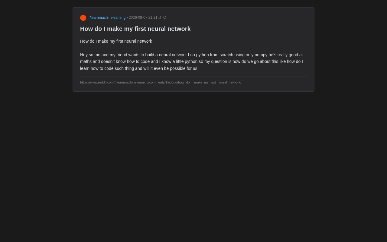
In Reddit's machine learning community, a beginner posed a very classic question: he and a friend with a strong math background wanted to build a neural network from scratch using only Python and NumPy. One person was good at math but couldn't code, while the other knew a bit of Python — could this duo actually pull it off?

The answer is: absolutely, and this is actually one of the most solid paths to learning deep learning.

Today, frameworks like PyTorch and TensorFlow have made neural network implementation incredibly simple — a few lines of code can train a model. But this comes with a side effect: many people have only a superficial understanding of the underlying principles. Building a neural network from scratch with NumPy means you have to write every line of code for forward propagation, backpropagation, and gradient descent yourself, which forces you to truly understand what a neural network is "actually doing."

NumPy (Numerical Python) is the most fundamental scientific computing library in the Python ecosystem, created by Travis Oliphant in 2005. It provides high-performance multidimensional array objects (ndarray) and a large collection of mathematical functions for array operations. NumPy's core advantage lies in its C and Fortran implementation under the hood, making vectorized operations tens to hundreds of times faster than pure Python loops. Before deep learning frameworks existed, NumPy was the tool of choice for researchers implementing machine learning algorithms. Even today, PyTorch's Tensor and TensorFlow's tensor APIs borrow heavily from NumPy's interface design. Understanding NumPy is truly the foundation for understanding all modern deep learning frameworks.

Prerequisites for Building a Neural Network

Math Fundamentals

The original poster's friend being strong in math is a huge advantage. The core mathematical foundations for building a neural network from scratch include:

• Linear Algebra: Matrix multiplication and vector operations form the backbone of neural networks. The computation at each layer is essentially matrix multiplication plus bias. Specifically, a fully connected layer with n input neurons and m output neurons has a weight matrix of shape m×n, and multiplying the input vector by the weight matrix is the most basic matrix-vector multiplication in linear algebra. Understanding matrix shapes, transposition, and broadcasting rules is a prerequisite for correctly implementing neural network code.
• Calculus: The core of backpropagation is the chain rule for computing derivatives. Understanding partial derivatives and gradients is key to mastering the training process.
• Probability and Statistics: Understanding the meaning of loss functions (like cross-entropy) and activation functions. The mathematical essence of cross-entropy loss comes from KL divergence in information theory — it measures the "distance" between the predicted probability distribution and the true distribution.

For someone strong in math, these concepts aren't difficult. The challenge lies in "translating" mathematical formulas into code.

Python Programming Requirements

The original poster only knows a bit of Python, and that's fine. Building a basic neural network doesn't require advanced programming skills. The main requirements are:

• Basic Python syntax (functions, loops, classes)
• NumPy array operations (especially np.dot, broadcasting, np.exp, etc.)
• Basic debugging ability

NumPy's broadcasting mechanism deserves special attention. Broadcasting is a set of rules in NumPy that allows arithmetic operations between arrays of different shapes — for example, adding an array of shape (3,1) to an array of shape (1,4) automatically "broadcasts" to produce a (3,4) result. This mechanism is ubiquitous in neural networks. For instance, adding a bias vector to every sample in a batch of data is a classic broadcasting operation. Understanding broadcasting rules helps avoid a multitude of shape-mismatch bugs.

The pair's combination is actually ideal: the math-savvy partner can derive formulas and verify logic, while the programmer handles implementation and debugging. This kind of "pair learning" is often more efficient than working alone.

Core Components of a Neural Network Explained

The simplest fully connected neural network consists of the following components. Understanding them means understanding the entire process.

Forward Propagation

Data flows from the input layer to the output layer. The computation at each layer follows this formula:

Z = W · X + b
A = activation(Z)

Here, W is the weight matrix, X is the input, b is the bias, and activation is the activation function (such as Sigmoid or ReLU). In NumPy, this is simply matrix multiplication.

Regarding activation function selection: The Sigmoid function (σ(x) = 1/(1+e^(-x))) was the standard choice for early neural networks, mapping any real number to the (0,1) interval. However, Sigmoid suffers from the "vanishing gradient" problem — when the absolute value of the input is large, the gradient approaches zero, making it difficult to train deep networks. After 2010, ReLU (Rectified Linear Unit, f(x) = max(0,x)) became the mainstream choice. It's computationally simple and has a constant gradient of 1 in the positive region, effectively mitigating the vanishing gradient problem. For beginners implementing with NumPy, it's recommended to start with Sigmoid (because its mathematical properties are elegant — its derivative can be expressed in terms of itself: σ'(x) = σ(x)(1-σ(x))), then transition to ReLU.

Loss Function

This measures the gap between predicted values and true values. Classification problems typically use cross-entropy loss, while regression problems use mean squared error (MSE). This is the objective function that the neural network optimizes.

The choice of loss function affects not only training speed but also the model's convergence behavior. For binary classification, although MSE is mathematically valid, cross-entropy loss produces larger gradients when predictions are severely wrong, pushing the model to correct errors faster. This is why classification problems almost always use cross-entropy rather than MSE — when paired with Softmax/Sigmoid output layers, the gradient has an elegant form (predicted value minus true value), and numerical stability is better.

Backpropagation

This is the hardest and most critical part. Using the chain rule, it computes the gradient of the loss with respect to each parameter, propagating layer by layer from the output back to the input. A math-savvy partner can play a tremendous role here.

The core of the backpropagation algorithm — the chain rule — is a fundamental theorem in calculus, but its systematic application to neural network training has a rather winding history. Although the mathematical form of backpropagation was proposed as early as the 1960s, it wasn't until 1986, when David Rumelhart, Geoffrey Hinton, and Ronald Williams published their landmark paper Learning representations by back-propagating errors, that the algorithm gained widespread recognition and spurred a neural network renaissance. The essence of the chain rule is decomposing the derivative of a composite function into the product of derivatives at each layer, which means that no matter how many layers a network has, all parameter gradients can be computed efficiently through layer-by-layer recursion, without needing to differentiate each parameter individually.

In NumPy implementations, a practical trick for backpropagation is "gradient checking": using numerical methods ((f(x+ε)-f(x-ε))/(2ε)) to approximate gradients and compare them with analytical gradients to verify the correctness of your backpropagation code. This is extremely effective for debugging common mistakes like matrix transposition errors and dimension mismatches in backpropagation.

Parameter Updates: Gradient Descent

Update weights using the computed gradients:

W = W - learning_rate * dW
b = b - learning_rate * db

Repeat this process thousands of times, and the network gradually learns.

The learning_rate here is one of the most important hyperparameters in neural network training. If the learning rate is too large, parameter updates overshoot, potentially causing the loss to oscillate or even diverge. If the learning rate is too small, training is extremely slow and can easily get stuck in local minima. In practice, researchers have developed numerous variants of gradient descent to address this issue: Stochastic Gradient Descent (SGD) updates using only one sample at a time — noisy but fast; Mini-batch SGD takes a middle ground, typically with a batch size of 32 or 64. Later, momentum-based SGD, AdaGrad, RMSProp, Adam, and other adaptive learning rate optimizers emerged. Among these, Adam (Adaptive Moment Estimation) combines the advantages of momentum and adaptive learning rates, making it one of the most commonly used optimizers in practice. For a NumPy beginner implementation, it's recommended to start with basic batch gradient descent, then try implementing momentum and Adam after understanding the principles.

Hands-On Roadmap: From Perceptron to MNIST Recognition

Step 1: Implement a Perceptron with NumPy

Don't jump straight into building a multi-layer network. Start by implementing a single neuron (perceptron) with NumPy to solve a simple binary classification problem, such as determining which side of a line a point falls on. This will help you get comfortable with the basic workflow of forward propagation and weight updates.

The Perceptron was proposed by Frank Rosenblatt in 1957 and is one of the earliest artificial neural network models. Its mathematical model is extremely simple: a weighted sum of input features passes through a step function (or sign function) to produce a binary classification output. Despite its simplicity, the Perceptron Convergence Theorem guarantees that for linearly separable data, the algorithm will find the correct classification hyperplane in a finite number of steps. Implementing a perceptron with NumPy might only require 20-30 lines of code, but those 20-30 lines contain the most essential logical framework of neural networks.

Step 2: Add Activation Functions and Hidden Layers

Implement a network with one hidden layer using Sigmoid or ReLU activation functions. The classic introductory task is solving the XOR problem — something a single-layer perceptron cannot do — which intuitively demonstrates the value of hidden layers.

The XOR (exclusive or) problem holds iconic significance in the history of artificial intelligence. In 1969, Marvin Minsky and Seymour Papert proved in their book Perceptrons that a single-layer perceptron cannot solve linearly inseparable problems like XOR. This finding directly led to the first "AI winter" for neural networks, with research funding slashed and academic interest plummeting. It wasn't until the 1980s, with the popularization of multi-layer networks and the backpropagation algorithm, that it was shown that a hidden layer with just two neurons could perfectly solve the XOR problem. Therefore, solving the XOR problem with your own code is not just a technical exercise — it's recreating a key breakthrough in the history of artificial intelligence.

Step 3: Train on MNIST Handwritten Digit Recognition

This is the "Hello World" of deep learning. Use your hand-built neural network to recognize handwritten digits from 0-9. While the accuracy may not match that of mature frameworks, the sense of accomplishment when you see your purely hand-written code actually recognizing digits is unparalleled.

The MNIST (Modified National Institute of Standards and Technology) dataset was created by Yann LeCun and colleagues in 1998, containing 70,000 grayscale images of handwritten digits at 28×28 pixels (60,000 for training, 10,000 for testing). These images were sourced from handwriting samples by U.S. Census Bureau employees and high school students. MNIST became the "Hello World" of deep learning because it's moderately sized (trainable without a GPU), the task is intuitive (everyone understands digit recognition), and there are clear performance benchmarks. A simple two-layer fully connected network can achieve roughly 97% accuracy, while current state-of-the-art models exceed 99.8%. It's worth noting that as the field has advanced, MNIST is now considered "too easy," and more challenging datasets like Fashion-MNIST and CIFAR-10 are gradually replacing it as the go-to entry-level benchmark.

When implementing an MNIST classifier with NumPy, keep a few practical details in mind: input images need to be flattened from 28×28 2D matrices into 784-dimensional 1D vectors; pixel values should be normalized to the [0,1] range (divide by 255); the output layer needs 10 neurons corresponding to the 10 digit classes, typically using the Softmax function to convert outputs into a probability distribution.

Step 4: Optimize and Extend

Add techniques like mini-batch gradient descent, learning rate scheduling, and regularization, and observe how they affect training performance.

Regularization is a critical technique for preventing neural network overfitting. The two most common approaches are L2 regularization (also called weight decay, which adds a penalty term proportional to the sum of squared weights to the loss function) and Dropout (randomly "shutting off" a subset of neurons during training). L2 regularization is very simple to implement in NumPy — just subtract an additional quantity proportional to the weights during gradient updates. Weight initialization strategies (such as Xavier initialization and He initialization) are equally crucial for training stability — initial weights that are too large or too small can cause gradient explosion or vanishing.

Recommended Learning Resources

For a project like building a neural network from scratch with NumPy, the community widely recommends several high-quality resources:

• Andrew Ng's Deep Learning Course: Covers everything from mathematical derivations to code implementation with great clarity, and includes assignments where you build a neural network from scratch with NumPy. This course is the "Deep Learning Specialization" series on Coursera, consisting of 5 courses. The programming assignments in the first course, Neural Networks and Deep Learning, involve implementing shallow and deep neural networks in pure NumPy — perfectly suited for the learning path discussed in this article.
• "Neural Networks and Deep Learning" (Michael Nielsen): A free online book implemented in Python with clear, in-depth explanations. A standout feature is its interactive visualizations to explain concepts, and the complete code implements a network achieving over 96% accuracy on MNIST in fewer than 100 lines.
• 3Blue1Brown's Neural Network Video Series: Explains backpropagation through visualization — an excellent supplement for those strong in math. Grant Sanderson's unique mathematical animation style makes abstract gradient flows visually intuitive.
• Andrej Karpathy's "micrograd" Project: A minimalist automatic differentiation engine in under 100 lines of code — a powerful tool for understanding backpropagation. Karpathy (former Tesla AI Director and OpenAI founding team member) walks through the code line by line in an accompanying YouTube video, starting from scalar-level automatic differentiation to show how the core ideas behind frameworks like PyTorch can be implemented with minimal code.

Practical Advice for Beginner Duos

First, this project is absolutely doable — don't be intimidated by "building from scratch." The core logic of neural networks is actually simpler than you might think. The real complexity lies in engineering optimization, and that's not something you need to worry about at the beginner stage.

Second, leverage your complementary strengths. The math-savvy friend should first derive the forward propagation and backpropagation formulas on paper, then both partners can work together to translate the formulas into NumPy code. Test with small data after completing each section to ensure correctness. A particularly effective collaboration approach: the math partner writes out the analytical gradient expressions for each layer, while the programming partner implements them and uses numerical gradient checking to verify correctness.

Finally, understand first, optimize later. The first version of your code doesn't need to be efficient or elegant — if it runs and produces correct results, that's a win. Once you truly understand the principles, transitioning to PyTorch will feel like an "aha" moment — you'll understand what every function in the framework is doing behind the scenes.

Modern deep learning frameworks like PyTorch and TensorFlow add three key capabilities on top of what NumPy provides: automatic differentiation (Autograd), GPU acceleration, and computational graph optimization. Automatic differentiation eliminates the need to manually write backpropagation code — the framework automatically tracks all operations and computes gradients. GPU acceleration parallelizes matrix operations through CUDA, potentially speeding up training by orders of magnitude. Computational graph optimization further improves efficiency through operator fusion, memory reuse, and other techniques. Once you've fully implemented a neural network with NumPy, when you use these frameworks, you'll deeply understand what happens behind loss.backward(), which parameters optimizer.step() updates, and why certain operations require detach() or no_grad() — these are no longer black magic, but automated versions of logic you've implemented by hand.

Conclusion

Building a neural network from scratch with NumPy is a rite of passage that every deep learning learner should experience. It not only builds a deep understanding of underlying principles but also cultivates the core ability to translate mathematics into code. For a duo where one knows math and the other knows programming, this is not only feasible — it's an ideal collaborative project. Get started now, beginning with a simple perceptron.

Key Takeaways