CNN Core Mechanisms Explained: From Convolution Principles to the Double Descent Phenomenon

In the self-study path of deep learning, Convolutional Neural Networks (CNNs) are often an unavoidable watershed. A learner systematically self-studying UC Berkeley's CS189 course recorded their understanding of CNNs on Day 11. These notes start from "why fully connected layers can't handle image tasks," build progressively, and ultimately touch on a phenomenon that still puzzles the academic community — Double Descent. This article uses these notes as a guide to outline CNN's core mechanisms and explore patterns in deep learning that remain incompletely explained.

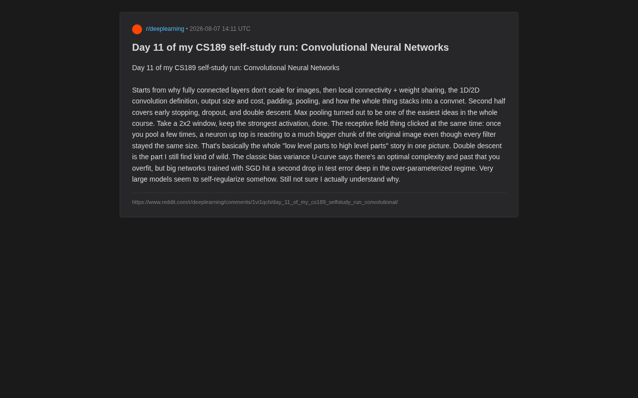
Why Do Image Tasks Need Convolution? The Limitations of Fully Connected Layers

The first step to understanding CNNs is understanding the limitations of Fully Connected Layers. Suppose we want to process an ordinary color image — say, a 224×224×3 input. If we directly connect it to a hidden layer with just 1,000 neurons using a fully connected layer, the parameter count instantly explodes to hundreds of millions. This scale is not only computationally expensive but also highly prone to severe overfitting.

In a fully connected layer, every neuron connects to all neurons in the previous layer. This "all-to-all" connection pattern is acceptable when processing one-dimensional feature vectors, but produces catastrophic parameter explosion when facing high-dimensional image data. Taking ImageNet's standard 224×224×3 input as an example, the flattened vector is 150,528-dimensional. If connected to 4,096 hidden neurons (as in VGGNet's fully connected layer design), this single layer alone requires approximately 616 million parameters. In comparison, the total convolutional layer parameters of the entire VGG-16 network amount to only about 14 million. Excessive parameters not only cause dramatic increases in memory usage and computation time but also give the model far more degrees of freedom than the data's information content, making it extremely easy to memorize noise in training samples rather than learning generalizable patterns.

Convolutional layers solve this problem through two key designs: Local Connectivity and Weight Sharing. Local connectivity means each neuron only attends to a small region of the input image rather than the entire image; weight sharing allows the same filter to slide across the entire image for reuse, drastically reducing the number of parameters.

The design inspiration for weight sharing partly originates from discoveries in visual neuroscience: simple cells in the mammalian primary visual cortex (V1) show selective responses to edges of specific orientations, and this response pattern remains consistent across different positions in the visual field. Mathematically, weight sharing makes the convolution operation equivalent to performing cross-correlation on the input signal — a fixed kernel extracts the same type of features at all spatial positions. This introduces an important inductive bias: translation equivariance, meaning that a translation of the input image causes an equal translation of the feature map without changing the detection results. This property makes CNNs naturally suited for visual recognition tasks where objects may appear at any position in the image.

From a mathematical definition perspective, whether 1D or 2D convolution, the essence is sliding a small kernel over the input and computing dot products. Around this operation, several engineering parameters need to be understood: how output size changes with stride and kernel size, how padding preserves edge information, and the overall computational cost. These details collectively determine the actual behavior of a convolutional layer.

Pooling and Receptive Fields: The Key from Local Features to Global Semantics

Max Pooling is straightforward: take a 2×2 window and keep the strongest activation value. Pooling reduces the spatial resolution of feature maps, decreases computation, and provides a degree of translation invariance.

What truly deserves deeper understanding is the connection between pooling and the Receptive Field. After several pooling operations, a neuron at the top layer is actually responding to a much larger region of the original image — even though the kernel size at each layer remains unchanged.

The receptive field size can be precisely calculated using a recursive formula: for layer L, the receptive field size is RF_L = RF_{L-1} + (k_L - 1) × ∏_{i=1}^{L-1} s_i, where k_L is the kernel size at layer L and s_i is the stride at layer i. This formula reveals a key insight: stride has a multiplicative amplification effect on the receptive field. Modern architectures like ResNet and EfficientNet carefully plan the growth curve of receptive fields during design, ensuring the final layer's receptive field covers the entire input image. Additionally, Dilated/Atrous Convolution exponentially expands the receptive field by inserting gaps between kernel elements without increasing parameters or performing pooling. This technique has been widely applied in semantic segmentation (e.g., the DeepLab series) and speech synthesis (e.g., WaveNet).

This is precisely the core of CNN's classic narrative of "from low-level to high-level features": shallow layers capture local details like edges and textures, and as receptive fields expand layer by layer, deeper layers begin to recognize more abstract, more global semantic structures. The entire hierarchical feature abstraction process can be summarized by the picture of "receptive fields expanding layer by layer."

Overall Architecture Stacking of Convolutional Networks

Repeatedly stacking convolutional layers, activation functions, and pooling layers, then attaching fully connected layers at the end for classification, constitutes a complete ConvNet. This structural modularity is the fundamental reason CNNs can efficiently process images — parameters are constrained within a reasonable range while preserving sensitivity to spatial structure.

Regularization Techniques: How Early Stopping and Dropout Prevent Overfitting

Early Stopping is a simple yet effective regularization method: terminate training when validation error begins to rise, preventing the model from overfitting on the training set. From an optimization perspective, early stopping is equivalent to limiting the distance parameters can move from the initialization point, and in a certain sense is equivalent to L2 regularization — a connection first theoretically established by Ali Rahimi, Benjamin Recht, and others, showing that early stopping actually imposes an implicit constraint in parameter space.

Dropout is more elegant. During training, it randomly "shuts off" some neurons with a certain probability, forcing the network not to rely on any single pathway, thereby learning more robust feature representations. Dropout was proposed by Hinton et al. in 2012, and its theoretical motivation can be understood from multiple perspectives. The most intuitive explanation is the ensemble learning perspective: randomly shutting off neurons each time is equivalent to sampling a sub-network from an exponentially large set of sub-networks for training, while using all neurons during inference (with weights scaled by the retention probability) is equivalent to approximately geometrically averaging the predictions of all sub-networks. Another perspective comes from information bottleneck theory: Dropout forces each neuron to independently learn useful features, preventing fragile "co-adaptation" relationships from forming between neurons. In practice, dropout rates are typically set to 0.5 (hidden layers) or 0.2 (input layers), and in convolutional layers, Dropout has been gradually replaced by Batch Normalization, as the latter usually provides better regularization effects in CNNs.

Both methods embody a core idea in deep learning practice: controlling the model's effective complexity is key to achieving good generalization ability.

The Double Descent Phenomenon: Why Do Over-Parameterized Models Generalize Better?

Classical bias-variance theory tells us there is a U-shaped curve between model complexity and test error: too low complexity leads to underfitting, too high leads to overfitting, with an "optimal complexity" in between. This theory has long dominated statistical learning intuition and is one of the most fundamental frameworks in machine learning textbooks, with roots traceable to Vapnik's VC dimension theory and the structural risk minimization principle.

However, large neural networks trained with SGD break this picture. When models enter deep into the over-parameterized regime, test error undergoes a second descent. That is, massive models with far more parameters than data points actually exhibit better generalization ability.

The double descent phenomenon was first systematically described by Belkin et al. in their 2019 paper Reconciling modern machine learning practice and the bias-variance trade-off. Subsequently, OpenAI's 2019 research confirmed that this phenomenon simultaneously exists along the model complexity dimension (increasing parameters), the training time dimension (extending training epochs), and the sample size dimension (increasing data). This means double descent is not an isolated experimental anomaly but a ubiquitous statistical phenomenon in deep learning.

The core paradox of this phenomenon lies in the fact that very large models seem to achieve self-regularization in some way. Current mainstream theoretical hypotheses include: (1) The implicit regularization hypothesis — the SGD optimizer naturally tends to find solutions with minimum norm, which typically have better generalization performance; (2) Interpolation threshold theory — at the critical point where the model can just barely perfectly fit the training data (interpolation threshold), the solutions satisfying the conditions in parameter space are extremely few and often have high variance, but upon entering the over-parameterized region, qualifying solutions form a rich manifold from which the optimizer can select smoother solutions; (3) The Neural Tangent Kernel (NTK) framework — in the infinite-width limit, neural network training is equivalent to kernel methods, and generalization behavior can be analyzed through the kernel's spectral properties. These hypotheses provide partial explanations from different angles but have not yet formed a unified theoretical framework.

This precisely reflects the current state of deep learning theory's frontier — the double descent phenomenon has been confirmed by extensive experiments, but theoretical explanations of its underlying mechanisms continue to evolve, involving multiple unsettled research directions including implicit regularization, optimization dynamics, and model interpolation capacity.

Summary: The Cognitive Path for Systematically Learning CNNs

The process of systematically learning CNNs condenses the typical cognitive trajectory of deep learning practitioners: some concepts (such as max pooling and convolution operations) are intuitive and instantly clear once understood; while others (such as the theoretical explanation of double descent) remain shrouded in mystery even after mastering the phenomenon itself.

For anyone systematically studying convolutional neural networks, the key lies in clearly distinguishing which aspects are firmly established engineering intuitions (local connectivity, weight sharing, receptive field expansion) and which remain open research questions (over-parameterized generalization, double descent mechanisms). Acknowledging "not yet fully understood" is itself the first step toward truly deep understanding.

Key Takeaways