Complete Guide to Vector Databases: From Embeddings to Semantic Search with ChromaDB

When a user searches for "how to improve focus" and the system returns documents that merely contain the word "focus," while an article that genuinely discusses "attention training" gets missed—this is the classic frustration of keyword search, and it's exactly the core problem vector databases are designed to solve. In a comprehensive beginner-friendly course, an instructor with ten years of software engineering experience and four years of AI engineering experience walks through the entire pipeline—from vectors, similarity, tokenization, and embedding models all the way to hands-on work with ChromaDB—breaking down each link in sufficient detail. This article distills the key threads and adds some practical perspectives.

What Problem Do Vector Databases Actually Solve?

The course's definition: a vector database is a database specifically designed to store, index, and search high-dimensional vector embeddings generated by embedding models, with semantic search as its core capability. Three concepts within this definition need to be unpacked: high-dimensional vector embeddings, embedding models, and semantic search.

Traditional relational databases excel at structured data—rows, columns, fixed schemas—with queries relying on WHERE clauses for exact matching or range filtering. But much of today's data is unstructured: text, PDFs, audio, video, images. These data have high dimensionality and are meaning-centric. Traditional databases can store them but struggle to retrieve them at scale based on meaning.

The key distinction lies between "keywords" and "semantics." Keyword search requires the query term to appear in the document; semantic search compares distances in vector space. The course's demonstration illustrates this well: after storing several sentences, querying with "programming" returns "how to write a Python function" and "how to create a class in Java"—neither of which contains the word "programming," yet both are highly relevant semantically. Querying with "electronics" returns "Apple releases new iPhone" and "which smartphone takes the best photos."

One point worth emphasizing: vector databases do not replace traditional databases. The course explicitly states that in real systems the two work together: the traditional database serves as the system of record, and the vector database builds a semantic retrieval layer on top of it. This judgment aligns with mainstream industry architecture.

From Vectors to Similarity: Understanding the Mathematical Foundation of Search

To understand vector databases, you must first understand vectors. In the context of machine learning, a vector is a one-dimensional array of numbers, where each number represents a feature of an object. The course uses cars as an example: with only the "speed" feature, it's a one-dimensional vector that can be plotted on a number line; adding "fuel consumption" makes it two-dimensional, plottable on a plane; adding "price" makes it three-dimensional, plottable in 3D space. With real embedding models, dimensionality can reach around 3,000—beyond human visualization—but the intuition that "similar items are close together in space, different items are far apart" always holds.

The course specifically clarifies a common misconception: not all vectors are vector embeddings. Vectors are a broader mathematical object; embeddings are vectors produced by embedding models that carry semantic meaning.

There are two primary measures of similarity. Cosine similarity considers only direction, not magnitude, with values ranging from -1 to 1: a result of 1 means the two vectors point in the same direction, 0 means they are orthogonal (no direct relationship), and -1 means opposite directions. The course demonstrates with vectors A=[2,0,1] and B=[4,0,2]: the dot product is 10, the magnitudes are 2.23 and 4.47 respectively, and the cosine similarity is approximately 1—even though B's magnitude is nearly twice A's, the same direction yields a high similarity judgment. This is precisely why cosine similarity suits vector embeddings: the semantics of an embedding are carried by direction, not magnitude.

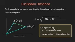
Euclidean distance, by contrast, measures the straight-line distance between two points in space, with values from 0 to infinity, where 0 means identical. It cares about "how far apart" and not about direction, making it more suitable for scenarios where physical distance is meaningful—GPS, robotics, spatial computing. The course's recommendation: in vector database and semantic retrieval scenarios, cosine similarity is the more commonly used choice.

Tokenization and Embedding: How Semantics Are "Computed"

Embedding models don't understand raw text; they first convert text into tokens. The course categorizes tokenization into three types: character-level, word-level, and subword-level. Character-level splitting is too fine-grained and causes token counts to explode; word-level splitting treats each word as an independent unit, inflating the vocabulary and failing to handle out-of-vocabulary words; subword-level splitting strikes a balance, breaking words into smaller reusable units.

The course uses OpenAI's tokenizer to demonstrate several typical phenomena: common words map to a single token, rare words are split into multiple tokens, Unicode characters like emoji may be split byte by byte into multiple tokens, and common numeric sequences like "123," "456," and "789" are merged into single tokens. For the same passage, character-level tokenization yields 252 tokens, while subword-level requires only 53. Modern large language models universally adopt subword tokenization, with the core motivation being to control token counts—and tokens are the basis for embedding model billing, so understanding tokens directly relates to cost.

After tokenization, the embedding model converts tokens into high-dimensional vectors. Here's a key insight: tokens themselves are just numeric symbols that carry no semantics; semantics are "encoded" into vector space during the embedding stage. The course uses vector arithmetic for an intuitive demonstration: king - man + woman ≈ queen, Delhi - India + Japan ≈ Tokyo. The model was never explicitly trained to perform such operations, yet the relationships between words are encoded as directions and displacements in vector space.

Subword tokenization deserves elaboration. Take the common BPE (Byte Pair Encoding) algorithm: starting from characters or bytes, it repeatedly counts the most frequent adjacent symbol pairs in the corpus and merges them into new symbols, ultimately producing a vocabulary that balances the integrity of common words with the decomposability of rare words. WordPiece and SentencePiece are different implementations of similar ideas; the latter also supports training directly on raw text without pre-splitting by spaces, making it friendlier to space-free languages like Chinese. The key value of subword tokenization lies in handling out-of-vocabulary words: word-level tokenization can only mark words unseen during training as unknown symbols, whereas subword tokenization can break them into known fragments—for example, splitting a rare word into a root plus affixes—from which the model can still derive partial semantics. This also explains the phenomena in the original demonstration where emoji are split by bytes and common numeric sequences are merged into single tokens—the tokenizer's merge rules are entirely determined by the statistical patterns of the training corpus.

Three Types of Embedding Models and How to Choose

The course divides embedding models into three generations. The first generation is word embeddings, represented by Word2Vec and GloVe, which take a single word as input and output a vector. The limitation is the loss of context: "bank" in "river bank" and "bank account" gets the same vector, unable to distinguish meaning.

The second generation is text embeddings, where the input can be a sentence, paragraph, or even an entire document, allowing direct comparison of semantic similarity between two texts. Vendors like OpenAI, Google Gemini, and Cohere all provide such models; they are the foundation of semantic search, RAG, and recommendation systems.

The third generation is multimodal embeddings, supporting both text and images. The course mentions Google's Gemini Embedding 2 supports text, images, video, audio, and even PDFs as input. The selection logic is straightforward: for pure text scenarios, text embeddings suffice; if the retrieval target is a PDF with mixed text and images, multimodal embeddings become necessary.

The course also mentions Microsoft's CodeBird, optimized for code understanding and used for code similarity and code search. This hints at an easily overlooked point: embedding models are diversifying by domain, and a general-purpose model may not be the optimal choice for a specific scenario.

The technical prerequisite for multimodal embeddings is mapping different modalities into the same vector space. A text encoder and an image encoder convert sentences and images into vectors respectively, with the training objective being that aligned image-text pairs are close to each other in space while unrelated pairs are far apart—typically achieved through contrastive learning. The result is that you can use text vectors to retrieve image vectors, commonly known as cross-modal retrieval. This differs from simply converting images into vectors as well: if each modality is trained independently, text and image vectors occupy different spaces, and their distances are not comparable. Therefore, when selecting a model, beyond checking whether it supports image input, you must also confirm that it outputs aligned vectors in a shared space. The image-text PDF scenario mentioned in the original article relies precisely on this property; otherwise, query text and image vectors in the document cannot be directly compared.

Inside a Vector Database: Four-Layer Architecture and Two Types of Indexes

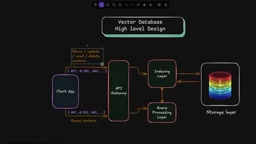
The course breaks down the internal structure of a vector database into four layers. The API gateway is the entry point, exposing CRUD operations and query interfaces for vectors; writes (ingestion phase) and queries are two different types of operations. The indexing layer organizes vectors to support efficient similarity search and avoid brute-force scanning. The storage layer handles persistence of high-dimensional vectors, emphasizing fast insertion, retrieval, and deletion, ensuring durability and fault tolerance through replication, and enabling scaling through partitioning. The query processing layer receives query vectors, coordinates the indexing and storage layers, and completes filtering and ranking.

The indexing layer is key to performance. The course focuses on two types of approximate nearest neighbor (ANN) indexes: IVF (Inverted File Index) and HNSW (Hierarchical Navigable Small World). Their common goal is to avoid linear scanning—with a million vectors, comparing one by one has linear complexity and unacceptable latency; ANN indexes trade approximation for speed, returning results in milliseconds. The course acknowledges that dedicated chapters will cover these algorithms in depth; here it only establishes a framework for understanding.

Approximate nearest neighbor (ANN) search is the core trade-off vector databases make between scale and latency. Exact nearest neighbor search requires comparing the query vector against every vector in the database one by one, with complexity O(N·d); when the number of vectors reaches millions and dimensionality reaches hundreds or thousands, the time per query cannot meet online service requirements. The ANN approach abandons "guaranteed to find the single global nearest" in favor of returning sufficiently close results with high probability, reducing query complexity to sublinear. In engineering, recall (the proportion of true nearest neighbors among returned results) is typically used to measure the loss introduced by this approximation. IVF partitions vectors into several inverted buckets via clustering, and queries scan only the most relevant buckets; HNSW builds a multi-layer navigable graph, performing greedy search layer by layer from a sparse top layer downward. The two avoid full scanning through "spatial partitioning" and "graph navigation," respectively. Understanding this is essential to grasping the later statement that index parameter tuning directly affects recall and latency.

Hands-On: Generating Embeddings with Gemini and Semantic Search in ChromaDB

The course's hands-on section has two steps. The first step uses the Gemini embedding model in Google Colab to generate vectors. The core call is client.models.embed_content, passing the model name (e.g., gemini-embedding-001), the content, and the configuration. The configuration specifies an output dimension of 768 and sets the task type to semantic similarity. The Gemini embedding model supports outputs from 128 to 3072 dimensions, with recommended dimensions of 768, 1536, and 3072. After generation, each sentence's embedding is a 768-dimensional array.

To intuitively verify the results, the course uses cosine similarity to compute a pairwise similarity matrix between sentences. The results match expectations: "how to write a Python function" and "how to create a class in Java" have the highest similarity; "which smartphone takes the best photos" and "what is the best Android phone" are highly similar; "turn off the light" matches "turn off the lights." Then PCA reduces the 768 dimensions to three for visualization, and Plotly creates an interactive 3D scatter plot where similar sentences clearly cluster in space.

The second step stores the embeddings in ChromaDB and queries them. The process: create a ChromaDB client and set a persistence directory; use get_or_create_collection to create a collection (analogous to a table in a relational database); write the embeddings, original document text, and IDs into the collection together. There's an easily overlooked but crucial constraint when querying: the query vector must be generated using the same embedding model and the same dimensionality as when writing. The course's exact words: if the model or dimensionality is inconsistent, the query simply won't work—because the query vector and the vectors in the database must be in the same vector space to be comparable.

In the demonstration, querying "programming" returns "how to write a Python function" and "how to create a class in Java"; querying "electronics" returns "Apple releases new iPhone" and "which smartphone takes the best photos." Neither query's keywords appear in the result texts, yet semantic matching works. This is both the value of semantic search and the underlying capability of applications like RAG, recommendation systems, and enterprise knowledge bases.

Learning Path and a Few Reminders

The course is positioned from zero to advanced, covering the complete pipeline from concepts to hands-on work, suitable for software engineers, AI engineers, and machine learning engineers. If I were to add a few practical reminders:

First, dimension selection requires balancing effectiveness and cost. Higher dimensions typically retain more information, but storage and computation overhead rise accordingly; 768 dimensions is already a reasonable starting point for most scenarios.

Second, the choice of similarity measure should fit the business. Cosine similarity suits semantic retrieval, Euclidean distance suits scenarios where physical distance is meaningful, and the two are not interchangeable at will.

Third, parameter tuning of index algorithms (IVF, HNSW) directly affects recall and latency. The course only lays the conceptual groundwork; actual projects need load testing based on data scale.

Fourth, ChromaDB is suitable for rapid prototyping and small-to-medium-scale scenarios; production-grade large-scale deployment requires evaluating distributed, replication, and partitioning capabilities. The course only introduces replication and partitioning at the storage layer in principle, and this area deserves deeper investigation during implementation.

Vector databases have become one of the foundational infrastructures of AI applications. Understanding their internal mechanisms has more long-term value than knowing how to call a few APIs.

One-line Summary

A systematic explanation of vector database principles and ChromaDB semantic search in practice, from vectors and similarity to tokenization and embedding models.

Paragraph Summary

The article systematically maps out the complete knowledge chain of vector databases: they are designed to store and retrieve high-dimensional vectors generated by embedding models, with semantic search as their core capability, and they complement rather than replace traditional databases. It starts with vectors and similarity measures, explaining that cosine similarity considers only direction and suits semantic retrieval, while Euclidean distance measures straight-line distance and suits physical-space scenarios. It then analyzes tokenization and embedding mechanisms, noting that subword tokenization controls token counts and that semantics are encoded into vector space during the embedding stage. It categorizes embedding models into three generations: word embeddings, text embeddings, and multimodal embeddings. Internally, a vector database consists of an API gateway, indexing layer, storage layer, and query processing layer, with IVF and HNSW being two key ANN indexes. The hands-on section uses Gemini to generate 768-dimensional embeddings and store them in ChromaDB, validating semantic matching that hits results even when keywords don't appear, and emphasizing that queries and writes must use the same model and dimensionality.