Convergence Analysis of High-Order ODE Solvers for Diffusion Models: Error Bounds and Fast Sampling Theory

From Generating Cat Images to the Mathematical Essence of Diffusion Models

At an MIT diffusion model seminar, MIT Mathematics CLE Moore Instructor Zhengzhang Lin presented a theoretical collaboration with Peking University Assistant Professor Zhengyu and Zhaoyang Huang (soon joining Iona) — a convergence analysis of high-order ODE solvers in diffusion probabilistic models. This work stands in sharp contrast to everyday image generation applications; it is pure theoretical mathematics, aimed at providing rigorous error guarantees for fast sampling methods from first principles.

The researchers opened with an intuitive example: suppose you have a collection of cat images and want to learn the true distribution over all cat images, enabling a sampler that generates a brand-new cat image from Gaussian noise each time. Ideally, if you could find a diffeomorphism mapping from a Gaussian distribution to the target distribution, the problem would be solved. The real challenge, however, is that images, audio, and video tend to be extremely high-dimensional, with data distributions that are neither smooth nor convex — just an unstructured cloud of random data.

The Forward and Reverse Processes of Diffusion Models

The mathematical foundation of diffusion models rests on the Ornstein-Uhlenbeck (OU) process. Originally proposed in 1930 by physicists Leonard Ornstein and George Uhlenbeck to describe the velocity evolution of Brownian particles subject to drag, the OU process differs from pure Brownian motion in possessing a mean-reverting property — the state is continuously pulled back toward an equilibrium point while random perturbations are superimposed. Its mathematical form is dXt = -αXt dt + σ dWt, where α is the reversion rate and Wt is standard Brownian motion. This property makes the OU process a natural choice for the forward noising step in diffusion models: with appropriate parameter settings, any initial distribution converges exponentially to the standard Gaussian in finite time, providing a controlled noise starting point for the reverse generation process.

The forward process uses a stochastic differential equation (SDE) to progressively add noise to a clean image until it becomes pure Gaussian noise. Equivalently, the noisy image Xt at any time can be expressed as a linear combination of the original image X0 and Gaussian noise, with normalization coefficients that keep the variance at one.

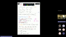
The true key lies in the reverse process — how to recover a high-quality original distribution from noise. The core driving force of the reverse process is the score function, the log-density gradient ∇x log p(x), which points in the direction of steepest increase in probability density. As early as 2005, Aapo Hyvärinen proposed Score Matching, which estimates probability models by minimizing Fisher divergence without computing the normalization constant. In diffusion models, a neural network is trained to predict the score function at various noise levels — a process equivalent to the denoising autoencoder objective. Yang Song et al.'s 2020 work proved that the forward SDE has a time-reversed counterpart SDE determined entirely by the score function, which is precisely why accurately learning the score function is the core bottleneck for diffusion model quality. Classical SDE denoising methods require 100 to 1000 steps to complete one reverse pass, which is far too slow for interactive applications. The reverse process can equally be described by an ODE continuity equation whose vector field vt is composed of x plus the log-density gradient (score function). This reverse ODE flow is the central object of this research.

From the ODE perspective, exact solution of the reverse flow requires two things: accurate initial data (a Gaussian distribution) and precise vector field evaluations along the way. In practice, neither can be perfectly satisfied — the initial condition is not a perfect Gaussian, and the vector field can only be approximately evaluated by a neural network at a finite set of discrete time points. These are the two core challenges that theoretical analysis must confront.

Why High-Order ODE Solvers Are More Efficient

To explain the acceleration principle, Lin reviewed the basics of numerical ODE solving. The simplest first-order Euler method retains only the linear term of the Taylor expansion, with a per-step error of order h². Heun's method (a second-order method) evaluates the vector field at two points and retains the quadratic term, reducing the per-step error to order h³. The more general Runge-Kutta methods are universal high-order solvers.

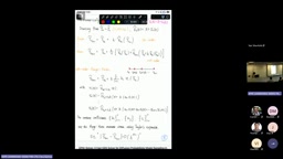
A key insight deserves emphasis: given the same available data, simply changing the update structure yields results much closer to the exact solution. An audience member raised a concern — don't high-order methods require more function evaluations, making them a trade-off? Lin's response was incisive: these vector field evaluations are actually collected during the forward noising process. However many steps the forward process takes, the reverse process can leverage that many steps of information. High-order methods therefore achieve higher fidelity in far fewer reverse steps.

This idea gave rise to widely used methods like DPM-Solver. Proposed by Cheng Lu et al. in 2022, DPM-Solver's core insight is to rewrite the reverse ODE of diffusion models as a semi-linear structure: the linear part is solved exactly, while the nonlinear part (the neural network's noise prediction) is handled with high-order numerical integration, fully exploiting the special algebraic structure of the diffusion ODE so that the exponential integrating factor can be computed analytically. Before this, DDIM had already reduced the sampling steps from 1000 to about 50; DPM-Solver compressed this further to roughly 10 steps, achieving an order-of-magnitude speedup over traditional SDE methods and making real-time image generation feasible. Exponential Runge-Kutta methods and various other improvements have since emerged, and fast ODE solving has become a highly developed engineering discipline.

Three-Term Error Decomposition and Two Core Challenges

The research team's goal was not to improve score function learning, but to quantify the final sampling error given an already well-trained neural network. They proved that the total variation (TV) distance between the learned and true distributions can be decomposed into three controllable terms. TV distance is defined as the supremum of the absolute difference between two probability measures: TV(P,Q) = sup_A |P(A) - Q(A)|. Compared to KL divergence, TV distance is symmetric and bounded (taking values in [0,1]), making it easier to manipulate in theoretical analysis and providing a clear mathematical connection to sampling quality. The three terms are:

• Initialization error: arising from the deviation of the initial distribution from a perfect Gaussian. Since the noised image is exponentially close to Gaussian, this term is very small;
• Score error: arising from the L2 distance between the neural network's learned score and the true score;
• Solver discretization error: arising from the discrete ODE solving itself, i.e., the order h^(P+1) error of Runge-Kutta methods.

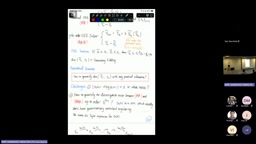
However, directly applying classical ODE theory faces two obstacles. First, classical ODE theory typically requires the vector field to be close in the L∞ norm (pointwise), but training only yields score error estimates in the L2 sense. Second, constructing high-order solvers via Taylor expansion implicitly requires the function to have very high regularity (C^(P+1)), which neural networks as vector fields cannot guarantee. These two issues put the theoretical validity of high-order error rates in question.

Verifying C2 Regularity for Neural Networks

For the second challenge, the research team took a notably practical approach: they actually trained diffusion models on the standard MNIST and Fashion-MNIST datasets and numerically verified whether the regularity assumptions on the neural network hold.

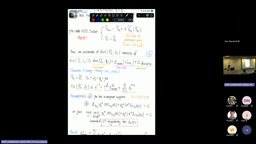
Their assumption does not require the bare Hessian norm to be small; instead, it uses a weighted form — sigma_t to the sixth power multiplied by the Hessian should be bounded by some constant. Experiments revealed that even when the Hessian itself reaches 300 on MNIST and 1000 on Fashion-MNIST, once multiplied by the normalization factor (where sigma_t is large in regions of high noise, i.e., near Gaussian), the result converges to a small constant (roughly order 1 to 2). This numerically confirms the practical reasonableness of the C2 regularity assumption and represents an important contribution distinguishing this work from prior studies — all estimates are based on information obtainable during actual training, without introducing additional artificial assumptions.

Ghost Flow: An Elegant Construction That Bypasses Low Regularity

How can one still obtain high-order discretization error when only C2 regularity is available, while Runge-Kutta theory requires C^(P+1) regularity? The team's key idea is to construct a "Ghost Flow."

Concretely, they use the true score function to construct a Ghost Flow driven by a Heun solver that runs in parallel with the learned flow. Through this intermediary, the TV distance between the learned-score flow and the true-score flow is decomposed into three segments: the first corresponds to initialization error (the difference in initial values between the two flows), the second corresponds to score error (same initial value, but driven respectively by the learned and true scores), and the third corresponds to discretization error (the difference between the true flow and its Heun discretization).

The elegance of this construction lies in the following: it transfers the regularity problem away from the low-regularity learned score onto the intrinsically smooth true score. The third error segment is built on the true (smooth) vector field, so Runge-Kutta theory can safely be applied to obtain an h^(P+1) error; the difficulty of low regularity is cleverly "absorbed" into the second score error term, where the triangle inequality and PDE estimates faithfully preserve the original L2-squared error.

Numerical experiments further show that the score error term dominates among the three error components, and the overall TV error in practice scales linearly with the score error. This means that if higher regularity assumptions on the learned score (such as C^K) can be established, sharper error dependence can be obtained.

Outlook: Broader Applications of High-Order Methods

In closing, Lin noted that the most inspiring takeaway of this work may not lie in diffusion models per se, but in the transferability of the high-order solver idea. The most immediate beneficiary is Flow Matching, which has attracted considerable attention in recent years. Proposed by Lipman et al. in 2022, Flow Matching directly learns a deterministic ODE flow mapping a noise distribution to the data distribution. Its mathematical structure is highly unified with the reverse ODE of diffusion models — both learn a vector field over a probability path — with the key difference being greater flexibility in the design of the interpolation path. The latest large-scale generative models including Stable Diffusion 3 and Meta's MovieGen have already shifted to flow matching frameworks, giving high-order solver theory direct industrial relevance. Any model that involves approximating some kind of flow can potentially leverage high-order methods to accelerate sampling and draw on analogous mathematical analysis strategies.

Of course, open theoretical questions remain: current error bounds exhibit dimension dependence (factors of d or d² appear in the error), which would need to be improved via low-dimensional manifold assumptions; moreover, convergence analysis for settings using heavy-tailed noise (rather than Gaussian noise) remains almost entirely unexplored. But for the broad class of flow-based generative models, both accelerated solving and convergence analysis remain fertile theoretical ground well worth cultivating.

Key Takeaways