Diffusion Models for Beginners: From DDPM Principles to UNet in Practice

From DDPM forward noising and reverse denoising to UNet code implementation, this article walks through the complete diffusion model pipeline and compares it with GANs.
Based on a video tutorial, this article systematically walks through diffusion models from DDPM theory to UNet code implementation. It contrasts GANs' unstable adversarial training and explains how diffusion models provide a more controllable generation path through noising and denoising; derives the closed-form forward process formula so x_t can be computed directly from x₀; explains how the reverse process uses Bayes' theorem to train a UNet to predict noise, with the mean expression and MSE loss; and introduces UNet architecture, time step positional encoding, sampling, and common questions, noting stable training but slow sampling—a necessary path to understanding modern image generation.
Diffusion models have become the dominant paradigm in image generation, but the dense mathematical derivations in the original papers often deter beginners. Based on a step-by-step video tutorial, this article walks through the complete pipeline from DDPM (Denoising Diffusion Probabilistic Models) forward noising and reverse denoising to the UNet code implementation, with comparisons to the pain points of GANs to help readers build an intuitive understanding.
From GAN to Diffusion Models: Why a New Paradigm Is Needed
Generative Adversarial Networks (GANs) improve generation quality through a game between a generator and a discriminator, but training is extremely unstable. The tutorial uses the metaphor of a "game shill" to explain this dynamic: the generator keeps upgrading to fool the discriminator, and the discriminator adjusts accordingly, trapping both sides in endless adversarial competition. This game causes the loss curve to fluctuate wildly, makes the model prone to learning biases or shortcuts, and limits diversity.
Diffusion models offer a more controllable path. They do not rely on adversarial training; instead, they decompose the generation process into two stages—"noising" and "denoising"—each with a clear mathematical form. According to the Bilibili creator's recollection in the tutorial, the concept of diffusion models was proposed in papers as early as 2015, but it only truly entered the public eye after the DALL·E series demonstrated stunning results.
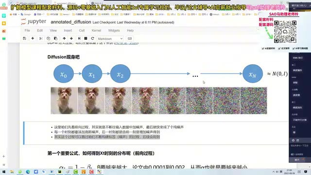
The Markov chain is the cornerstone of the mathematical framework of diffusion models. It describes a sequence of states in which each state depends only on the previous state and is independent of earlier history—a property called the Markov property. In diffusion models, each noising step of the forward process is modeled as a Markov transition: given x_{t-1}, the distribution of x_t is determined solely by the transition kernel q(x_t | x_{t-1}) and is conditionally independent of x_{t-2} and earlier states. It is precisely this property that allows the joint distribution of the entire noising chain to be factorized into a product of stepwise transition probabilities, thereby providing mathematical convenience for deriving the closed-form marginal distribution q(x_t | x₀) and the variational lower bound. The reverse process is likewise modeled as a Markov chain, learning the transition from x_t to x_{t-1}. Understanding the Markov property is a prerequisite for understanding the derivation of the DDPM loss function.
Forward Process: Gradually Turning an Image into Noise
The forward process is a fixed Markov chain: starting from the original image x₀, a small amount of Gaussian noise is added at each step, and after T steps we obtain pure noise x_T. The tutorial emphasizes that the noise variance is controlled by a preset β_t schedule, where β_t increases over time, meaning more noise is added later in the process.
The key derivation is that the distribution of x_t at any time step can be computed directly from x₀ and t without step-by-step iteration. The formula is:
x_t = √(ᾱ_t) · x₀ + √(1 - ᾱ_t) · ε
where ᾱ_t is the cumulative product of α_t = 1 - β_t, and ε is standard Gaussian noise. This property greatly simplifies training: the model can randomly sample a t and directly construct x_t without simulating the full chain. The tutorial uses the metaphor of a "Sanya tourist" to illustrate the progressive nature of noising: at the beginning, a small amount of noise can significantly change the image, but later more noise is needed to mask the signal.
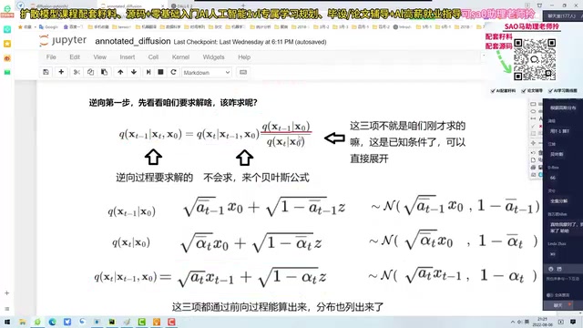
The β_t schedule is a key hyperparameter in the forward process that controls the pace of noising. β_t is a predefined sequence of small positive numbers that does not participate in training, typically growing linearly or cosinely from β_1≈1e-4 to β_T≈0.02. It determines the variance of the Gaussian noise added at each step, which in turn affects the signal retention ratio through α_t = 1 - β_t and the cumulative product ᾱ_t. If β_t is too small, noising is too slow and T must be very large to reach pure noise; if β_t is too large, the image structure is destroyed early and the model struggles to learn fine-grained denoising. The original DDPM used a linear schedule, while later work (e.g., Nichol & Dhariwal) proposed a cosine schedule that makes the decay of ᾱ_t smoother and performs more stably on both low- and high-resolution images. The choice of schedule directly affects generation quality and training convergence speed.
Reverse Process: Reconstructing an Image from Noise
The goal of the reverse process is to learn p(x_{t-1} | x_t), i.e., to predict the distribution of the previous step given a noisy image. Theoretically, this conditional distribution can be transformed into the form of the forward process using Bayes' theorem, but it contains a term that cannot be computed directly—the noise ε.
The tutorial derives the expression for the mean μ_θ:
μ_θ(x_t, t) = (1/√α_t) · (x_t - (β_t / √(1 - ᾱ_t)) · ε_θ(x_t, t))
where ε_θ is the neural network to be trained, which takes x_t and t as input and outputs a prediction of the noise. The variance is set to a fixed value in the original DDPM, but the tutorial notes that later improved versions allow the variance to be learned as well.
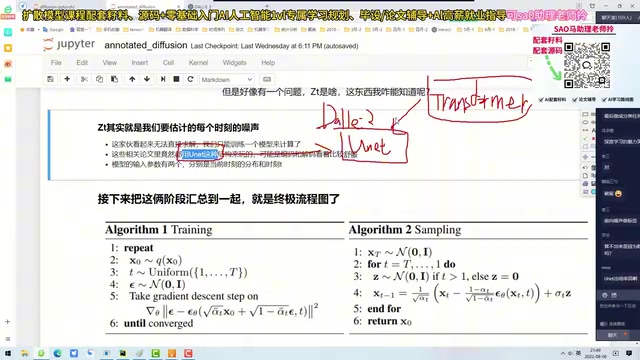
Training and Sampling: How UNet Learns to Predict Noise
The core of the training phase is to make the UNet predict noise. The specific procedure is: sample x₀ from the dataset, randomly choose a time step t, sample noise ε, construct x_t, and then have the UNet output ε_θ; the loss function is the mean squared error ||ε - ε_θ(x_t, t)||². The tutorial code uses the Fashion-MNIST dataset; the UNet input consists of x_t and the positional encoding of t, and the output is a noise prediction of the same size as the input.
The sampling phase starts from pure noise x_T, iteratively calls the trained UNet to predict noise, computes x_{t-1} according to the formula, and gradually denoises until x₀. The tutorial sets T=200 in the code (the original paper used 2000) and demonstrates the generation process on CPU. Although the generated results are not perfect, the outlines of clothing are already visible.
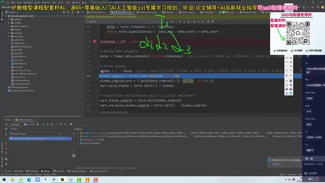
Positional encoding is used in diffusion models to let the network perceive the time step t. Since the convolution operations of the UNet themselves have no concept of time steps, the scalar t must be converted into a high-dimensional vector and injected into the network. DDPM follows the sinusoidal positional encoding from the Transformer: for each time step t, a set of fixed-dimensional embedding vectors is generated using sine and cosine functions of different frequencies, then mapped through two fully connected layers to a dimension matching the number of feature map channels, and finally used to modulate the features of each layer via element-wise addition or FiLM. This encoding enables the network to distinguish different noise levels and thus adopt different denoising strategies for early (strong signal) and late (strong noise) stages. The quality of the time step embedding has a significant impact on generation results, and later work has also explored variants such as learnable embeddings.
Key Implementation Points and Common Questions
The UNet architecture includes downsampling, a middle block, and upsampling; the time step t is embedded via sinusoidal positional encoding and then added to the feature maps. The tutorial specifically mentions that the additional attention mechanism in the UNet is puzzling, and the author speculates that it may have been added merely to increase novelty. Regarding the question "why can't T be backpropagated?", the tutorial explains that the sampling operation itself is non-differentiable, but during training the loss function is a regression on the noise prediction, so gradients can be backpropagated normally.
The choice of dataset directly affects the generated content: when the input is pure noise, the model reconstructs the most common categories in the training set. The tutorial recommends that beginners start with small datasets (such as Fashion-MNIST) to gradually understand the principles before attempting larger-scale tasks.
The value of diffusion models lies in their clear mathematical framework and stable training characteristics. Although sampling is slow, subsequent improvements (such as DDIM and latent diffusion) continue to push them toward practicality. For researchers who want to dive deep into generative models, starting with DDPM is a necessary path to understanding modern image generation systems.
One-line Summary
From DDPM forward noising and reverse denoising to UNet code implementation, this article walks through the complete diffusion model pipeline and compares it with GANs.
Paragraph Summary
Based on a video tutorial, this article systematically walks through the complete pipeline of diffusion models from DDPM theory to UNet code implementation. It first contrasts the instability of adversarial training in GANs and explains how diffusion models provide a more controllable generation path through two stages—noising and denoising; then it derives the closed-form formula for the forward process, allowing x_t at any time step to be computed directly from x₀; next it explains how the reverse process can be transformed via Bayes' theorem into training a UNet to predict noise, and gives the mean expression and mean squared error loss; finally it introduces the UNet architecture, time step positional encoding, the sampling procedure, and common questions, noting that diffusion models train stably but sample slowly, and that they are a necessary path to understanding modern image generation systems.
Related articles

How Did Da Vinci Prove the Sun Is Hot? A Neglected Chapter in Science History
How did da Vinci use a concave mirror experiment to overturn Aristotle's cold sun theory? This article traces this neglected chapter in science history, revealing the embryo of scientific thinking in the 15th century and da Vinci's cold observations on solar heat and the nature of life.
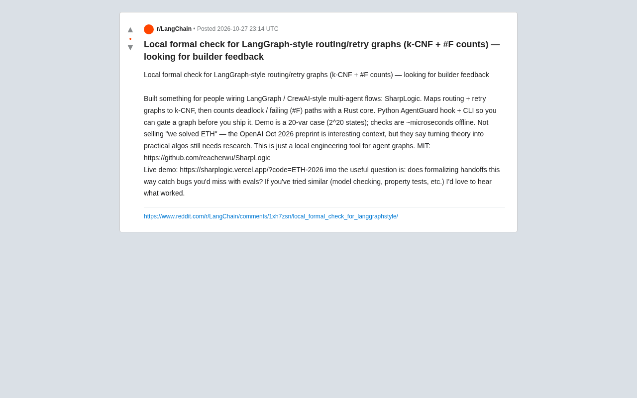
SharpLogic: Formalizing Bug Detection for LangGraph Routing Graphs with k-CNF
SharpLogic, an open-source project, maps LangGraph-style multi-agent routing and retry graphs to k-CNF, using a Rust kernel to count deadlocks and failing paths (#F counting), offering a Python AgentGuard hook and CLI for pre-release formal gate checks. This article analyzes its principles, its complementary relationship with evals, and the community's concern about modeling costs.
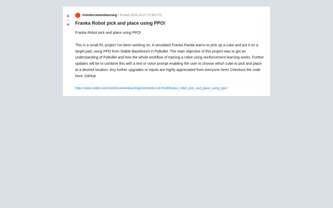
PPO Training of a Franka Robotic Arm for Pick-and-Place: A Reinforcement Learning Starter Project
A reinforcement learning project using PPO to train a Franka Panda robotic arm for pick-and-place in PyBullet, covering tech stack choices, task design challenges, and future text/voice command interaction plans—a good reference for beginners.