Diffusion Models from Scratch: A Complete Derivation from Adding Noise to Denoising

Diffusion models replace the GAN game with noising and denoising, with noise prediction and closed-form solutions at the core.
This article systematically explains diffusion models and why they replaced GANs: GANs' two-network game is hard to train with volatile losses, while diffusion models have the clear objective of predicting noise. It covers the forward noising process and closed-form solution, the reverse denoising process via Bayes' formula and neural network noise prediction, the training and sampling pipeline, UNet structure and time-step encoding, Fashion-MNIST code highlights, and the Gaussian premise, approximation error, and extensions.
Title
Diffusion Models from Scratch: A Complete Derivation from Adding Noise to Denoising
Meta Description
A beginner-friendly explanation of diffusion model principles: starting from the limitations of GANs, fully deriving the forward noising and reverse denoising formulas, explaining why a neural network is needed to predict noise, with UNet structure and code implementation highlights.
The heat around Generative Adversarial Networks (GANs) is fading, and the Diffusion Model has become an unavoidable name in the field of generative models. Since the DALL·E series brought this direction into the spotlight, understanding the principles and formulas of diffusion models has become a fundamental skill for understanding modern image generation technology. Based on a systematic explanation by a Bilibili creator, this article organizes the core logic of diffusion models in full—from adding noise and denoising to code implementation—while trying to avoid the derivation steps that are omitted in the papers.
Why Diffusion Models Replaced GANs
The idea behind GANs relies on a game between a generator and a discriminator: the generator tries to fool the discriminator, and the discriminator tries to tell real from fake. This adversarial mechanism brings several practical problems. The training process involves optimizing two networks simultaneously, making convergence difficult; the loss value fluctuates back and forth, making it hard to judge how good the training is; and the model may learn shortcuts that the trainer did not anticipate, resulting in reduced diversity of generated results.
Diffusion models take a different approach: first gradually add noise to an image step by step until it becomes pure noise, then train a model to learn to denoise and restore it step by step. Compared with the two-network game of GANs, its training objective is clearer—predict the noise added at each step. This idea is not new; similar papers appeared as early as 2015, but it did not truly attract large-scale attention until DALL·E 2 demonstrated stunning results in 2022.
According to the Bilibili creator's analysis, the rise of diffusion models is directly related to DALL·E 2 being built on diffusion models; some researchers have also admitted that after seven or eight years of work in the GAN direction, the room left to explore is getting narrower, and diffusion models have become the new main direction.
Markov chain is the basic mathematical framework for understanding the forward and reverse processes of diffusion models. It refers to a sequence of states in which each state depends only on the previous state and is independent of earlier states. The forward process of a diffusion model is exactly such a Markov chain: x_t is determined only by x_{t-1} and is conditionally independent of x_{t-2} and earlier states. This property allows the transition probability of each step to be written separately and also facilitates the later derivation of a closed-form solution. The reverse process is likewise modeled as a Markov chain, meaning that when restoring x_{t-1} from x_t, it depends only on the state at the current moment. It is worth noting that, strictly speaking, the reverse process can be approximated as a Markov chain only when the number of noising steps is sufficiently large and the noise at each step is sufficiently small, which is one reason diffusion models require relatively many steps.
Forward Process: From Image to Pure Noise
How Much Noise to Add at Each Step
The forward process is simply continuously adding noise to an image until the original distribution completely disappears. The key point is that the amount of noise added at each step is not the same: in the early stage, the image has clear structure, and adding a little noise can noticeably change the distribution; in the later stage, the image is already close to pure noise, and adding the same small amount of noise produces almost no visible change. Therefore, a time-dependent weight \beta_t that increases at each moment is needed to control the noising magnitude. The paper gives a value range of roughly 0.001 to 0.002, increasing linearly.
Define \alpha_t = 1 - \beta_t. Then the recurrence relation at each moment can be written as: x_t is jointly determined by the previous moment x_{t-1} and a standard Gaussian noise, each with its own weight coefficient. As time t increases, the weight of the previous moment decreases and the weight of the noise increases.
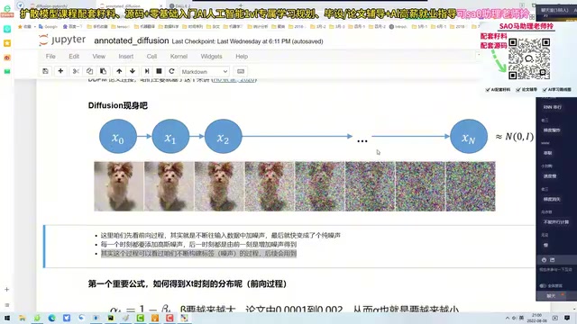
Directly Computing Any Moment from x0
If you honestly compute step by step according to the recurrence, it becomes a serial structure similar to an RNN, which is slow to compute and difficult for gradient propagation. A key contribution of the original paper is the derivation of a closed-form solution: the distribution of x_t at any moment can be expressed directly from the initial image x_0, without going through every intermediate step.
The derivation method is to repeatedly substitute the recurrence relation of adjacent moments and combine like terms. The noise terms are all standard Gaussian distributions; when two independent Gaussian distributions are added, their variances add directly. Therefore, after merging multiple times, a unified expression can be obtained: x_t equals the cumulative product of the square roots of \alpha_t multiplied by x_0, plus the square root of one minus the cumulative product of \alpha_t multiplied by a standard Gaussian noise.
This formula means that, given the initial image and the number of steps to which you want to diffuse, you can directly compute the noisy state at that moment without saving the intermediate process.
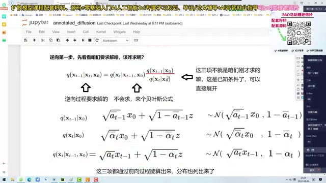
Reverse Process: Restoring the Image from Noise
Building a Bridge with Bayes' Formula
The problem the reverse process needs to solve is: given x_t, find the distribution of x_{t-1}. It cannot be solved directly, but the forward direction from x_{t-1} to x_t is known, so Bayes' formula can be used for conversion, turning the difficult conditional probability into the product of three computable terms.
After expanding these three terms, each corresponds to a Gaussian distribution. By completing the square and combining like terms, the mean expression of x_{t-1} can be obtained—it depends on both x_t and x_0. Here a key contradiction appears: x_0 is exactly the target we want to find, so it cannot be treated as a known condition.
Two key properties of Gaussian distributions support almost all derivations in diffusion models. First, the sum of two independent Gaussian distributions is still a Gaussian distribution, with means added and variances added—this is precisely the fundamental reason the forward process can merge multiple noising steps into a one-step closed-form solution. Second, given a Gaussian distribution, if a linear transformation is applied to it and independent Gaussian noise is added, the result is still a Gaussian distribution, which allows the conditional distribution of the reverse process to be parameterized in Gaussian form. In addition, when "completing the square" for the variance in the reverse derivation, the technique used is also completing the square for Gaussian distributions: separating the mean and variance to obtain an explicit expression of the mean in terms of x_t and x_0. Understanding these two properties makes the many omitted like-term-merging steps in the paper no longer mysterious.
Using a Model to Predict Noise
The solution is to express x_0 in reverse using x_t and substitute it into the mean formula. After rearranging, it turns out that the mean depends only on x_t and a noise term z_t, but z_t itself cannot be computed directly—we only know the current x_t and do not know what noise was added at each previous step.
The way scientists handle this is: since the formula cannot be derived, let a neural network predict this noise. Train a model that takes x_t and time t as input and outputs an estimate of the noise. Model training requires labels, and the labels happen to come from the forward process—the random noise generated when adding noise is itself known and can be saved directly as the ground truth. The loss function is the difference between the predicted noise and the true noise.
The variational lower bound (ELBO) is the theoretical source of the diffusion model training loss. Strictly speaking, a diffusion model is a latent variable model, and directly maximizing the log-likelihood is infeasible, so instead its variational lower bound is maximized. Through derivation, the ELBO can be decomposed into a sum of KL divergences across multiple moments, each measuring the difference between the reverse predicted distribution and the true posterior distribution. The original paper further simplified it and found that when the variance of the reverse process is fixed, optimizing these KL divergences is equivalent to minimizing the mean squared error between the predicted noise and the true noise. This explains why the final loss function has such a concise form—it is not designed out of thin air, but is the result of variational inference after simplification. Only by understanding this layer can one see that the seemingly intuitive choice of "predicting noise" has a rigorous theoretical basis.
Training and Sampling Pipeline
In the training stage, sample x_0 from the dataset, randomly select a moment t for each sample, add noise according to the forward formula to obtain x_t, let the UNet predict the noise, compute the loss, and backpropagate to update parameters. Randomizing the moment t is important to prevent the model from learning only the patterns of a fixed number of steps.
In the sampling stage, start from pure noise. At each step, use the trained UNet to predict the noise, combine it with the coefficients of the current moment to compute the mean, then add a scaled noise sample to obtain x_{t-1}, looping until the image is restored. The trained UNet shares parameters across all moments; only the input changes each time.
UNet Structure and Time-Step Encoding
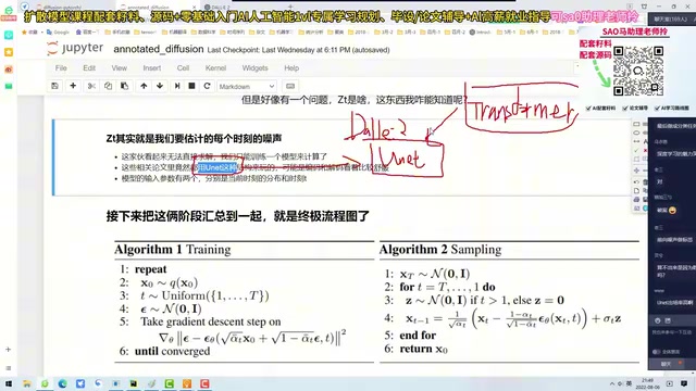
The main body of the model uses a UNet: first downsample to extract features, pass through several convolutional layers in the middle, then upsample and concatenate features from corresponding layers. The time t is converted into a vector through sine-cosine encoding similar to Transformer positional encoding, then added to and fused with image features, so that the network knows which noising stage it is currently in.
The Bilibili creator specifically mentions a phenomenon: diffusion models could clearly use a larger Transformer structure, yet the paper chose a UNet, and even added a simple attention module inside the UNet, the reason for which is not fully explained in the paper. A reasonable guess is that the task itself only needs to predict noise and does not require overly complex network capacity.
Positional encoding is often underestimated in diffusion models. The moment t is a scalar; if input directly into the network, the model has difficulty distinguishing subtle differences between adjacent moments. Sine-cosine encoding maps t to a high-dimensional vector; sine and cosine functions of different frequencies give each moment a unique pattern, and nearby moments have similar encodings, making it easier for the network to generalize smoothly to unseen steps. This is consistent with the idea of handling word-order positions in Transformers, except that diffusion models encode only one time dimension. The encoded vector usually passes through two fully connected layers and an activation function, then is injected into each residual block of the UNet via element-wise addition or concatenation, enabling each layer of features to perceive which stage of noising it is currently in.
Key Code Implementation Points
Using a grayscale image dataset such as Fashion-MNIST with 28×28 images, the full pipeline can run even on an ordinary CPU. In the implementation demonstrated by the Bilibili creator, the total number of diffusion steps is set to 200, \beta increases linearly from 0.001 to 0.002, and coefficients such as \alpha_t and its cumulative product, and the square root of one minus the cumulative product, are precomputed and directly looked up during training and sampling.
In the training loop, each batch is randomly assigned moments, then noise is added, prediction is performed, loss is computed, and parameters are updated. The sampling loop iterates in reverse order starting from t equal to the last step, calling the UNet each time to predict noise and compute the distribution of the previous step. Saving intermediate results allows you to see the process by which the image gradually reveals clothing outlines from pure noise.
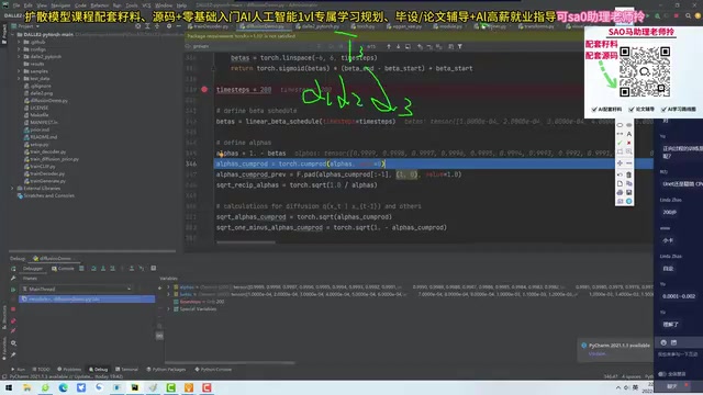
The Bilibili creator also mentions that he was initially baffled when looking at the paper's formulas, and only straightened things out by first understanding the code and then going back to fill in the mathematics. For readers with an average mathematical background, this order may be more effective than grinding through the paper.
Boundaries and Extensions of Diffusion Models
This basic framework has clear premises: the noise must follow a standard Gaussian distribution; deriving with other distributions would be much more difficult. If the training data itself does not conform to the Gaussian assumption, the applicability of the model will also be limited.
Each step of the reverse process contains approximations, and the predicted noise cannot be completely accurate, so the final generated result will differ from the original image. This is also why generation quality depends on model capability.
The extensibility of diffusion models goes beyond image generation. By replacing the input from random noise with text feature vectors, text-to-image generation becomes possible, and the DALL·E series succeeded precisely along this direction. The Bilibili creator mentions that training such large models requires extremely high computational power, making personal reproduction very difficult, but the principles are already clear.
As for the original paper, the Bilibili creator suggests that readers with an average mathematical background should proceed cautiously: the original paper unfolds from the perspectives of probability theory and information entropy, with many intermediate derivations omitted, and direct reading can easily get stuck in local formulas. First build an overall framework by following accessible explanations, then go back and compare with the paper—this will be much more efficient.
One-line Summary
Diffusion models replace the GAN game with noising and denoising; the core is predicting noise and training efficiently with the help of a closed-form solution.
Paragraph Summary
This article systematically organizes the core principles of diffusion models and explains why they replaced GANs: GANs' two-network game is difficult to train and has volatile losses, whereas diffusion models have the clear objective of predicting noise and are easier to converge. The article details how the forward process gradually adds noise and uses a closed-form solution to directly compute the state at any moment, how the reverse process uses Bayes' formula for conversion and a neural network to predict noise, and the training and sampling pipeline. It also introduces the role of the UNet structure and time-step encoding, provides key code implementation points based on Fashion-MNIST, and discusses the Gaussian noise premise, approximation error, and extensions toward text generation and other directions.
Related articles

How Did Da Vinci Prove the Sun Is Hot? A Neglected Chapter in Science History
How did da Vinci use a concave mirror experiment to overturn Aristotle's cold sun theory? This article traces this neglected chapter in science history, revealing the embryo of scientific thinking in the 15th century and da Vinci's cold observations on solar heat and the nature of life.
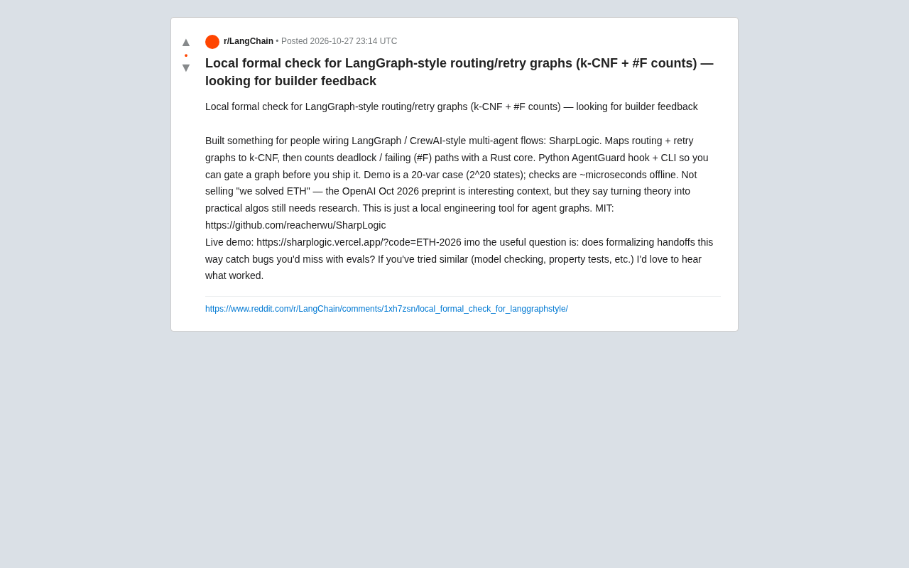
SharpLogic: Formalizing Bug Detection for LangGraph Routing Graphs with k-CNF
SharpLogic, an open-source project, maps LangGraph-style multi-agent routing and retry graphs to k-CNF, using a Rust kernel to count deadlocks and failing paths (#F counting), offering a Python AgentGuard hook and CLI for pre-release formal gate checks. This article analyzes its principles, its complementary relationship with evals, and the community's concern about modeling costs.

PPO Training of a Franka Robotic Arm for Pick-and-Place: A Reinforcement Learning Starter Project
A reinforcement learning project using PPO to train a Franka Panda robotic arm for pick-and-place in PyBullet, covering tech stack choices, task design challenges, and future text/voice command interaction plans—a good reference for beginners.