EI Algorithm's Three Design Choices Get First Theoretical Backing: Convergence Rates Guide Simulation Optimization

In continuous simulation optimization, the Expected Improvement (EI) method based on Stochastic Kriging (SK) surrogate models is widely used. But this approach has long faced an awkward reality: the noise level of simulation outputs is typically unknown and heteroscedastic, while the three core design choices of the EI algorithm—the current best value used to define "improvement" (the incumbent), the number of replications per sampled point (replication level), and the final recommended point (terminal recommendation)—all depend heavily on these unknown noise levels.

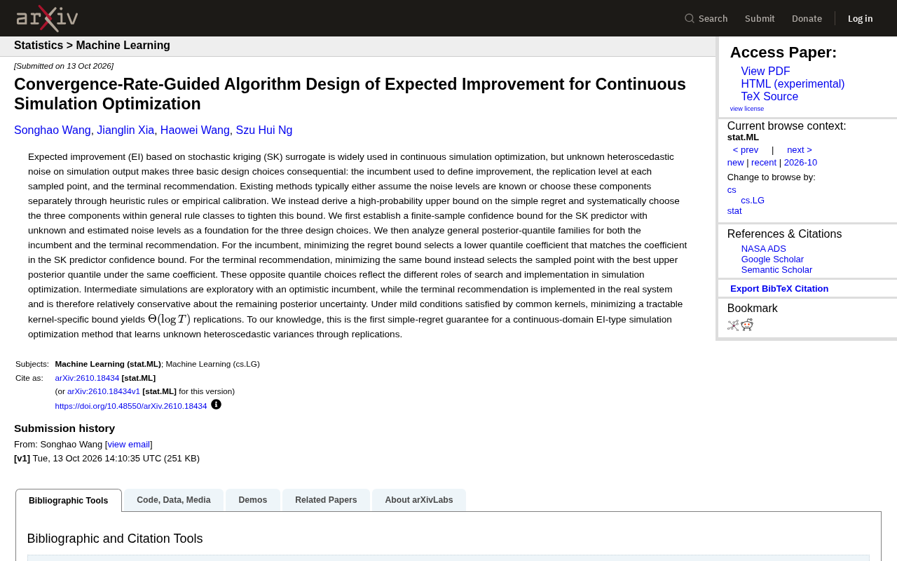
Existing approaches either assume the noise level is known or select these three components separately through heuristic rules or empirical calibration. A recent research paper breaks this deadlock: the researchers derive high-probability upper bounds on simple regret and systematically select the three components within a general rule class to tighten that bound. This is claimed to be the first simple regret guarantee for continuous-domain EI-type simulation optimization methods, and it can learn unknown heteroscedastic variances through replication.

Why the Three Design Choices Matter So Much

The core logic of the EI method is not complicated: fit a surrogate model to simulation outputs, then select the point with the greatest expected improvement for the next simulation. But in simulation scenarios where noise is unknown, every step becomes tricky.

The incumbent determines the baseline for "improvement." Choose it too optimistically, and the algorithm over-explores; choose it too conservatively, and it may converge prematurely to a suboptimal solution. The replication level is equally a dilemma—too few replications and noise drowns out the signal; too many and the computational budget is wasted. The terminal recommendation is the final answer delivered to decision-makers, and its quality directly determines the practical value of the entire optimization process.

The paper points out that these three choices are typically handled in isolation in existing methods, lacking a unified theoretical framework for guidance.

Stochastic Kriging (SK) is a generalization of ordinary Kriging surrogate models to noisy scenarios. Ordinary Kriging assumes observations are noise-free, with the interpolating surface passing strictly through all sample points; Stochastic Kriging instead models each observation as "true function value + random noise," so the predictor outputs not only a mean estimate but also a posterior variance. This distinction is crucial in simulation optimization: simulation outputs are inherently noisy, and forcing a noise-free Kriging fit would overfit to the noise. Stochastic Kriging typically assumes noise follows a Gaussian distribution and distinguishes between "homoscedastic" (same noise variance at all points) and "heteroscedastic" (different noise variances across points). This paper confronts the latter—noise variance is unknown and varies with input location, which is precisely the root cause making the three EI design choices difficult to handle uniformly.

Expected Improvement (EI) is a classic acquisition function in Bayesian optimization. Given the posterior distribution of the surrogate model and the current best value (incumbent), EI computes "the expected improvement relative to the incumbent that could be achieved by sampling at a candidate point." The intuition is that points with high posterior mean (likely better) or large posterior variance (more informative) both receive high EI values, naturally balancing exploration and exploitation. EI typically has a closed-form expression and is computationally efficient, making it widely adopted in continuous simulation optimization. But when the noise variance is unknown, the comparison involving the incumbent in EI is itself noisy, requiring additional replication and estimation mechanisms to support it—precisely the difficulty discussed in this article.

Reverse-Engineering Algorithm Design from Regret Bounds

The researchers' approach is "begin with the end in mind": first establish finite-sample confidence bounds for the SK predictor when the noise level is unknown and must be estimated, using this as the theoretical foundation for the three design choices.

Subsequently, they analyze a general posterior quantile family for the incumbent and terminal recommendation. The key finding is: when minimizing the regret upper bound, the incumbent should use a lower quantile coefficient, and this coefficient exactly matches the coefficient in the SK predictor's confidence bound; the terminal recommendation should select the sampled point with the best posterior upper quantile under the same coefficient.

These two seemingly contradictory quantile choices actually reflect the different roles of "search" and "implementation" in simulation optimization. Intermediate simulation steps are exploratory, and an optimistic incumbent helps thorough search; the terminal recommendation must be implemented in the real system, so it remains relatively conservative about remaining posterior uncertainty.

Simple regret is a metric measuring the quality of an optimization algorithm's final recommended solution, defined as the difference between the true function value of the optimal solution and the true function value of the algorithm's recommended solution. In contrast, cumulative regret measures the accumulated loss of every decision throughout the search process. Simple regret cares about "how good the final answer is," and simulation optimization is often oriented toward one-shot decisions—finding an optimal set of parameters and delivering them for implementation—making simple regret the more appropriate evaluation criterion. This paper derives a high-probability upper bound on simple regret, i.e., "with probability at least 1−δ, the regret does not exceed some expression in terms of the number of rounds T." Such guarantees are stronger than bounds in expectation and more capable of guiding concrete design.

Posterior quantile refers to the function value corresponding to a particular quantile in the surrogate model's posterior distribution. Choosing an upper quantile means adopting a more optimistic estimate (believing the true value may be higher), while choosing a lower quantile is more conservative. The paper's core insight is precisely to use quantile coefficients to uniformly characterize the incumbent and terminal recommendation: the incumbent takes a lower quantile to maintain search optimism, while the terminal recommendation takes an upper quantile to remain conservative about remaining uncertainty. The quantile coefficients match those in the SK confidence bound, making the three design choices self-consistent within the same theoretical framework.

Theoretical Solution for Replication Level

Under mild conditions satisfied by common kernel functions, minimizing a tractable kernel-specific upper bound yields a replication level of Θ(log T).

The significance of this result is that it provides a theoretical growth rate for the replication level rather than relying on empirical tuning. Logarithmic growth means that as simulation rounds increase, the number of replications per point grows slowly, giving computational resource allocation a theoretical basis.

The paper emphasizes that this guarantee is achieved by learning the unknown heteroscedastic variance through replication, rather than assuming the variance is known or pre-estimated.

The notation Θ(log T) comes from asymptotic complexity analysis: Θ indicates the same order for upper and lower bounds, meaning the replication level neither grows faster nor slower than log T—they are of the same order. In the context of simulation optimization, this means that as the total number of simulation rounds T grows, the replications allocated to each sampled point need only increase at a logarithmic rate. Logarithmic growth is extremely slow: for example, when T grows from one thousand to one million (about a thousandfold), log T only increases by roughly a factor of two. This explains why the conclusion has practical value: it shows that there is no need to invest a proportionally growing simulation budget for each new point—the marginal resource investment can be very restrained, providing algorithm designers with a clear basis for budget allocation.

Mild conditions typically refer to standard assumptions such as the kernel function being sufficiently smooth and eigenvalues decaying at a polynomial rate. These are routine prerequisites for convergence rate analysis of kernel methods, ensuring the SK predictor's confidence bound is controllable. The resulting Θ(log T) conclusion, while not holding for arbitrary kernels, covers commonly used Gaussian kernels, Matérn kernels, and others, giving it broad applicability.

Theoretical Contributions and Practical Significance

The most direct contribution of this work is filling the gap in theoretical guarantees for continuous-domain EI-type simulation optimization methods. Previously, similar regret guarantees existed mostly in discrete domains or settings with known noise.

From a practical standpoint, this framework provides clear guidance for algorithm designers: the incumbent and terminal recommendation should adopt quantiles in different directions rather than using the same set of heuristic rules. This design philosophy of "optimistic search, conservative delivery" may influence how future simulation optimization tools are implemented.

Of course, the paper's theoretical results rest on mild conditions satisfied by common kernel functions, and performance in more complex noise structures or non-stationary scenarios still requires further validation. But regardless, bringing three previously isolated design choices into a unified convergence rate analysis framework is itself a methodological advance.

One-line Summary

The paper provides the first simple regret guarantee for continuous-domain EI-type simulation optimization, unifying the determination of the incumbent, replication level, and terminal recommendation.

Paragraph Summary

This research addresses the long-standing theoretical gap in continuous simulation optimization methods based on Stochastic Kriging surrogate models with Expected Improvement (EI): simulation noise is unknown and heteroscedastic, and the three core design choices of EI—the incumbent, replication level, and terminal recommendation—all depend on these unknown noise levels. By deriving finite-sample confidence bounds for the SK predictor when noise must be estimated, and then analyzing the general posterior quantile family for the incumbent and terminal recommendation, the researchers find that when minimizing the regret upper bound, the incumbent should take a lower quantile (optimistic search) while the terminal recommendation should take an upper quantile (conservative delivery)—opposite directions. Under common kernel function conditions, the optimal growth rate for the replication level is Θ(log T). This is the first simple regret guarantee for continuous-domain EI-type simulation optimization methods, bringing three previously isolated design choices into a unified convergence rate analysis framework, and it can learn unknown heteroscedastic variances through replication.