Finite-Sample Bounds for Wide Neural Network Gaussian Approximation Lifted to Functional Convergence

Randomly initialized neural networks of width $m$ converge to a Gaussian process as $m \to \infty$. This conclusion is a theoretical cornerstone for understanding the training dynamics and generalization behavior of wide neural networks, but quantitatively characterizing the convergence rate has long involved a tension between two technical routes.

The Trade-off Between Two Types of Quantitative Bounds

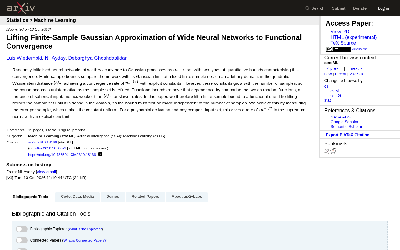
According to the original paper, existing quantitative bounds fall into two categories. Finite-sample bounds compare the network with its Gaussian limit on a fixed, finite sample set, apply to arbitrary input domains, adopt the quadratic Wasserstein distance $\mathcal W_2$, achieve a convergence rate of $m^{-1/2}$, and have explicit constants. But the paper explicitly points out that these constants grow with the number of samples, and as the sample set is progressively refined, the bounds become uninformative.

Functional bounds, by contrast, eliminate the dependence on the number of samples by comparing the two as random functions. The cost is that one must restrict to spherical inputs, use a weaker metric than $\mathcal W_2$, or accept a slower rate. Each route makes its own sacrifice: one is precise at fixed points but cannot be refined, while the other is general in function space but comes with stringent conditions.

Gaussian process limit: As the width m of a neural network tends to infinity, if the weights are randomly initialized in a particular way (e.g., independent and identically distributed, with variance scaled by 1/m), the joint distribution of the network outputs converges to a Gaussian process. The covariance function of this Gaussian process is determined by the network architecture (activation function, depth, initialization scheme). This limit is the foundation of neural tangent kernel (NTK) theory and a prerequisite for understanding why wide networks can be approximately characterized by kernel methods.

Wasserstein distance: $\mathcal W_2$ is a metric for measuring the difference between two probability distributions, based on optimal transport theory. For one-dimensional or Gaussian distributions, $\mathcal W_2$ has a closed-form solution; in high dimensions, it is weaker than total variation distance or KL divergence, but more sensitive to the geometric structure of the distributions. Finite-sample bounds commonly use $\mathcal W_2$ because it can directly compare the finite-dimensional distributions of network outputs and Gaussian processes, and it facilitates obtaining explicit constants. However, the convergence of $\mathcal W_2$ depends on the number of sample points, and when the sample set is dense, its constants diverge.

The Core Idea of the Lifting: Error per Sample

The core operation of the paper is to "lift" finite-sample bounds into functional bounds. The specific approach is to refine the sample set until it is dense over the domain. At this point, the bound must first be independent of the number of samples; otherwise, the refinement process would cause the constants to diverge.

The authors achieve this by measuring "error per sample," keeping the constants consistent. For polynomial activation functions and arbitrary compact input sets, this lifting yields a rate of $m^{-1/2}$ under the supremum norm with explicit constants. This means that the generality of functional bounds and the rate and explicit constants of finite-sample bounds can be obtained simultaneously, at least under the conditions of polynomial activations and compact domains.

Supremum norm: Defined as $|f|\infty = \sup{x \in \mathcal X} |f(x)|$, it measures the maximum deviation of a function over its entire domain. In function spaces, the supremum norm is stronger than $L^2$ or $\mathcal W_2$ because it requires simultaneous approximation at all points. Lifting finite-sample bounds to the supremum norm means that the entire sample path of the network converges uniformly to that of the Gaussian process, which is stronger than pointwise convergence or weak convergence and therefore more practically valuable. However, obtaining convergence under the supremum norm typically requires more refined tools, such as chaining or Dudley entropy bounds.

Compact input set: Compactness (equivalent to being bounded and closed in Euclidean space) guarantees the uniform continuity of continuous functions and makes the finite covering lemma applicable. In the lifting process, compactness allows us to approximate the entire domain with a finite grid, thereby controlling the error under the supremum norm. For non-compact domains, such as all of $\mathbb R^d$, uniform convergence typically does not hold and requires additional weighting or growth conditions.

Why This Lifting Is Noteworthy

From a theoretical perspective, this result bridges the gap between the two types of bounds. Previously, obtaining $m^{-1/2}$ rates with explicit constants at the function level typically required additional assumptions or accepting a weaker metric. The error-per-sample perspective provides a reusable technical tool: converting sample-count-dependent constants into uniform constants.

From a practical perspective, the Gaussian process approximation of wide neural networks is a theoretical pillar for directions such as Bayesian neural networks and neural tangent kernels. Improvements in quantitative bounds directly affect judgments about the behavior of these methods at finite width. When the sample set is dense, the previously uninformative bounds no longer apply, while the new bounds remain valid under the supremum norm, providing a tighter characterization of the gap between finite and infinite width.

Applicable Boundaries and Open Questions

It should be noted that the result currently targets polynomial activation functions and compact input sets. For more general activation functions, the original paper does not assert whether the error-per-sample method can still yield explicit constants. Additionally, whether the $m^{-1/2}$ rate under the supremum norm holds under weaker regularity conditions remains for future work.

This lifting is itself a highly technical result, but the idea it embodies—eliminating sample-count dependence by reorganizing the error metric—may have implications for other convergence analyses that need to transition from discrete comparisons to continuous ones.

One-line Summary

By measuring error per sample, the paper lifts finite-sample Gaussian approximation of wide networks to functional convergence, achieving $m^{-1/2}$ rates with explicit constants under polynomial activations and compact domains.

Paragraph Summary

This article discusses two types of quantitative bounds for Gaussian process approximation of wide neural networks: finite-sample bounds converge at rate $m^{-1/2}$ on fixed point sets but have constants that grow with sample count and become uninformative as the sample set is refined; functional bounds eliminate sample-count dependence but require restricting to spherical inputs, using a weaker metric, or accepting a slower rate. The paper proposes measuring error per sample to make the constants independent of sample count, thereby lifting finite-sample bounds to functional bounds. For polynomial activation functions and compact input sets, this lifting achieves $m^{-1/2}$ rates with explicit constants under the supremum norm, bridging the gap between the two types of bounds. This technical tool can be reused for other discrete-to-continuous convergence analyses and provides tighter finite-width characterizations for directions such as Bayesian neural networks and neural tangent kernels.