Google EmbeddingGemma 2 Local Deployment Guide: Four-Modality AI Search in Practice

One Model to Search Across Text, Images, Video, and Audio

Google's latest EmbeddingGemma 2 is a locally deployable multimodal AI search model. Its standout feature is a unified 768-dimensional shared vector space that maps text, images, video, and audio into a single semantic framework. This means you're no longer matching files by keyword — you're retrieving content by semantic similarity. Search images with text, find videos using images, locate audio with video clips: any cross-modal combination is possible.

According to hands-on testing shared by Bilibili creator 超哥, the model supports over 100 languages, handles up to 8K context length, and the model file itself weighs in at just 1.49GB — small enough to run on virtually any ordinary computer. For users who manage large local multimedia libraries, this lightweight cross-modal search tool offers real practical value.

Vector space and semantic similarity are the key concepts for understanding this tool. Traditional search relies on keyword matching — a file only turns up if its name or tag contains the word "cat." Vector retrieval works differently: the model compresses each piece of text, each image, and each audio or video clip into a fixed-length sequence of numbers (a vector). The more similar two pieces of content are, the closer their vectors sit in mathematical space. "768-dimensional" means each vector has 768 components — higher dimensionality generally allows the model to capture richer semantic detail. When all four modalities share the same vector space, a photo of a cat and a text description of a cat get mapped to nearby positions, making cross-modal retrieval possible. Closeness between vectors is typically measured using cosine similarity, which ranges from 0 to 1 — the closer to 1, the more semantically similar the two items are. This is what "similarity approaching 1.0" means in the test results below.

Real-World Testing: Where Semantic Search Shines

To validate the model's cross-modal capabilities, a test folder was assembled containing 27 items: 8 text files, 7 images, 6 videos, and 6 audio clips — roughly split between "cat" and "dog" content.

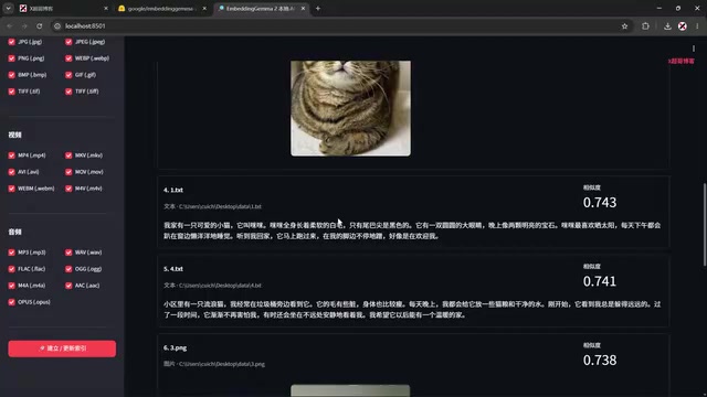
Searching for "cat" returned cat videos first, followed by cat-related text and cat images, while dog content was pushed to lower positions due to lower similarity scores. The critical point: none of those video or image files had "cat" or "dog" labeled in their filenames or tags — the model still identified the content and retrieved it accurately. This is the core advantage of semantic vector retrieval over traditional keyword search: it understands the content itself, not just file names or metadata.

Search results can be filtered further to show only text, images, video, or audio. In reverse image search mode, uploading a cat photo retrieves matching cat videos. When using a video file as the query, the selected video scores near 1.0 and ranks first, with other similar content sorted by descending similarity. Audio search performance is slightly weaker — when audio features are ambiguous (e.g., dog barks without other cues), similarity judgments can occasionally be off — but overall it remains functional.

Since results are ranked by similarity, the minimum similarity threshold and number of results settings directly affect recall quality and are worth paying attention to when using the tool.

Before Deployment: Downloading the Model and Setting Up the Environment

The full deployment process consists of four main steps. Step one is downloading the model and project files. The model is hosted on HuggingFace — published just one day prior — and all files, including the 1.49GB model file, need to be downloaded. Since downloading individual files is tedious, 超哥 has packaged everything into a cloud drive (available via Quark or Thunder), so you can grab the entire folder in one go.

Step two is installing the Python environment. Download the Python installer, double-click to run it, make sure to check "Add to PATH", then click Install Now. Once installation is complete, open CMD and type the verification command. If a Python version number (e.g., 3.12.0) appears, the environment is ready.

Configuring the Virtual Environment and Installing Dependencies

Step three is configuring the local search model — this involves the most commands in the entire process. Execute them in order:

Creating and Activating a Virtual Environment

1. Create a new folder on a drive of your choice (e.g., D:), using the name provided in the tutorial;
2. Move all files downloaded from the cloud drive into this folder;
3. Click the address bar in the folder, type cmd, and press Enter to open a command prompt in that directory;
4. Run the command to create the virtual environment — a corresponding folder will appear in the directory;
5. Run the activation command — when the command prompt prefix changes to a specific style, the environment is active.

Upgrading pip and Installing Dependencies

With the environment active, run the following in sequence: upgrade pip → install the GPU version of PyTorch → run the detection command (seeing True and your GPU name confirms CUDA is available) → install project dependencies. Once all dependencies are installed, the configuration stage is complete.

One thing to watch for: there is a typo in the tutorial where pip is written as ppp in one command — just correct it when you encounter it. Installing the GPU version of PyTorch means the model can leverage GPU acceleration, which is one reason search responses are fast.

Python virtual environments are the standard approach for isolating dependencies across different projects. Different AI projects often require specific library versions, and installing everything directly into the system Python can cause version conflicts. A virtual environment acts like a dedicated "sandbox" for the project — packages installed inside it don't affect the global system environment and aren't interfered with by other projects. When a virtual environment is activated, the command prompt prefix changes (usually displaying the environment name), which is the key indicator that you're working in the correct environment. The GPU version of PyTorch (CUDA build) is what enables the model to use NVIDIA GPU parallel computing — CPUs are relatively slow at vector operations, while GPUs have thousands of compute cores that can significantly speed up index building and retrieval. Seeing True and your GPU name after running the detection command confirms that the CUDA driver and PyTorch are properly connected.

Launching and Using the Tool: Choosing the Right Folder Is Key

Step four — launching — is straightforward. Navigate to the folder you created and double-click start.bat. Important note: do not close this terminal window — the web interface will stop working if you do. After launching, a browser window will open automatically with the search interface.

On first use, click "Select Folder" — the model will automatically build an index for that folder. One important warning: do not select your entire C: drive or system drive. System files are numerous, and indexing them will consume enormous amounts of time and disk cache. It's best to index specific media folders only.

The main controls in the interface include: query type (text / image / video / audio), search target (all modalities or a single one), the search bar, and a three-dot menu for theme switching and clearing cache. When the contents of a folder change, click "Update Index" to rebuild. After indexing, the system automatically tallies file counts by modality, and recently used folders are saved for quick access next time.

Who Is This For?

EmbeddingGemma 2 has a clear positioning: local, lightweight, and cross-modal. It doesn't upload data to the cloud, protecting your privacy. Its 1.49GB footprint keeps hardware requirements low. And its real killer feature is letting you query any modality using any other modality.

For photographers, video creators, asset managers, or anyone who wants to quickly locate content within a large personal file library, this is a tool worth trying. That said, it has limitations — audio recognition accuracy drops when audio features are ambiguous, and the deployment process involves Python environments and command-line operations, which may present a barrier for users with no technical background. Overall, for an open-source model released just one day ago, this local multimodal search experience is genuinely impressive.