How Likelihood Tempering Rescues Bayesian Neural Networks from 'Prior Collapse'

When Width Grows, Why Does Variational Inference Break Down?

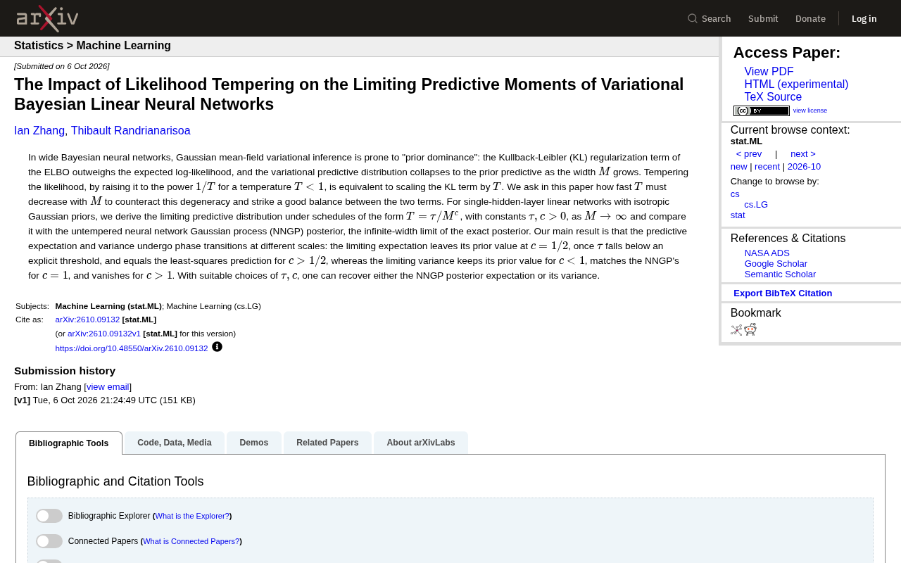
Bayesian Neural Networks (BNNs) aim to equip deep learning predictions with quantifiable uncertainty. In practice, however, Gaussian mean-field variational inference (mean-field VI) suffers from a long-standing problem known as prior dominance.

This new arXiv paper (arXiv:2610.09132v1) focuses precisely on this phenomenon. As network width $M$ grows, the KL divergence regularization term in the ELBO (Evidence Lower Bound) increasingly overwhelms the expected log-likelihood term. In other words, the wider the model, the more the training data's influence on the posterior is diluted — and the variational predictive distribution eventually degenerates into the prior predictive distribution, leaving the network unable to learn meaningful information from the data.

This is an awkward situation: in theory, wider networks should have greater expressive power, yet within the variational Bayes framework, width actually becomes a liability that degrades prediction quality.

Mean-Field Variational Inference (Mean-Field VI) is the most commonly used approximate inference strategy in variational Bayes: it assumes the posterior can be factorized into a product of independent distributions over each parameter, with each parameter independently following a Gaussian (parameterized by mean and variance). This dramatically reduces computational complexity but sacrifices the ability to capture correlations between parameters. ELBO (Evidence Lower Bound) is the optimization objective for variational inference, taking the form $\text{ELBO} = \mathbb{E}_q[\log p(\mathcal{D}|\theta)] - \text{KL}(q(\theta) | p(\theta))$, where the first term encourages the model to fit the data, and the second (KL divergence) pulls the approximate posterior $q$ toward the prior $p$. As network width $M$ grows, the number of parameters scales linearly, so the KL term (a sum of KL divergences over all parameters) also grows linearly, while the expected log-likelihood term grows more slowly. This causes the regularization term to dominate optimization — the fundamental mathematical reason behind prior dominance.

Likelihood Tempering: Rebalancing Two Forces with a Single Parameter

The core tool proposed in this paper is likelihood tempering. The approach is straightforward: raise the likelihood function to the power $1/T$, where temperature $T < 1$.

The key mathematical equivalence is this — tempering the likelihood is equivalent to multiplying the KL term in the ELBO by a factor of $T$. Since the problem stems from an overly strong KL term, using a $T < 1$ to downweight the KL term allows the expected log-likelihood to regain influence.

But the real challenge isn't whether to temper — it's how fast to temper. As width $M$ grows, prior dominance intensifies. If temperature decays too slowly, the KL term still dominates; if it decays too fast, regularization is excessively weakened. The paper's central question is: at what rate must $T$ decay with $M$ to strike the right balance between the two terms?

Phase Transitions: Expectations and Variances 'Jump' at Different Scales

To obtain analytically tractable results, the authors restrict their analysis to single-hidden-layer linear networks with isotropic Gaussian priors. They consider temperature schedules of the form $T = \tau/M^{c}$ (where $\tau, c > 0$ are constants), derive the limiting predictive distribution as $M \to \infty$, and compare it against the NNGP (Neural Network Gaussian Process) posterior — which is the form the exact posterior takes in the infinite-width limit.

The most striking finding is that the predictive mean and variance undergo 'phase transitions' at different scales — they do not transition simultaneously.

Phase Transition for the Predictive Mean

For the limiting predictive mean:

• When $c = 1/2$ and $\tau$ falls below a specific threshold, the mean begins to deviate from the prior;
• When $c > 1/2$, the limiting mean equals exactly the least-squares prediction.

In other words, the mean transitions at the scale $c = 1/2$: when temperature decays fast enough, the model recovers the optimal data-driven linear prediction.

Phase Transition for the Predictive Variance

The variance transitions at a different point:

• When $c < 1$, the variance remains at its prior value;
• When $c = 1$, the variance exactly matches the NNGP posterior variance;
• When $c > 1$, the variance vanishes.

The mean transitions at $c = 1/2$, while the variance only transitions at $c = 1$ — this offset dual phase transition is the paper's core contribution. It reveals a fundamental difference in how likelihood tempering affects the first and second moments of the predictive distribution.

The NNGP (Neural Network Gaussian Process) posterior serves as the "ideal target" for comparison in this paper. When network width tends to infinity under specific initialization conditions, the network's function-space distribution converges to a Gaussian process whose kernel is determined by the network architecture and activation function. For a finite dataset, the exact Bayesian posterior under NNGP is also a Gaussian process with analytically computable mean and covariance, representing "perfect" Bayesian inference in the infinite-width limit. The paper uses the NNGP posterior's mean and variance as a yardstick for measuring the quality of the variational approximation: the closer the variational predictive distribution is to the NNGP posterior, the more successfully likelihood tempering has "rescued" the mean-field approximation from prior dominance and brought it closer to true Bayesian inference.

Practical Implications: Recover What You Care About

This set of results yields an operationally useful corollary: by appropriately choosing $\tau$ and $c$, one can selectively recover either the NNGP posterior's mean or its variance.

This is a sobering reminder for practitioners — likelihood tempering is not a "magic switch" that can simultaneously and costlessly restore all statistical properties of the exact posterior to a mean-field variational approximation. If you care more about point prediction accuracy (the mean), the required schedule differs from the one needed when you care more about uncertainty quantification (the variance). To recover both simultaneously requires careful calibration in the parameter space.

From a methodological standpoint, the paper's value lies in elevating an empirical intuition — "tuning the temperature can alleviate prior collapse" — into a analytically grounded theory with explicit thresholds and scaling rates. Although the analysis targets the simplest possible setting (single-hidden-layer linear networks), it provides a clean mathematical reference frame for understanding degeneracy phenomena in more general variational Bayesian deep learning.

Limitations and Future Directions

It is worth acknowledging that the paper's conclusions rest on fairly idealized assumptions: a single hidden layer, linear activations, and an isotropic Gaussian prior. Whether the same dual phase transition pattern holds for real deep nonlinear networks remains an open question. But as many infinite-width network theories (such as NTK and NNGP) have demonstrated, analytically tractable linear and infinite-width models often reveal qualitative patterns that continue to hold in more complex settings.

For researchers focused on uncertainty quantification in Bayesian deep learning, this work delivers at least one clear message: temperature is not something to tune arbitrarily — its decay rate determines whether you end up with the prior, with a least-squares solution, or with a genuine approximation to the posterior.

NTK (Neural Tangent Kernel) is another important theoretical framework for infinite-width networks: when network width tends to infinity and learning rate tends to zero, gradient descent training can be exactly described by a fixed kernel function (the NTK), and network training becomes equivalent to kernel regression. Together, NTK and NNGP form the two main theoretical pillars for understanding the behavior of infinite-width neural networks — the former characterizes training dynamics, the latter characterizes Bayesian inference. Although these theories face practical challenges (finite width, nonlinear activations, mismatches between theoretical assumptions and actual training), their qualitative predictions often align closely with empirical observations in finite-width networks, making them widely used as analytical tools. This paper's analysis of single-hidden-layer linear networks follows the same tradition: extracting insights from analytically tractable extremes that can guide understanding of more complex models.