Introduction to Machine Learning: Core Concepts of Supervised Learning, Classification, and Featurization Explained

Introduction: Understanding Machine Learning from Scratch

Machine learning is becoming an essential skill for technology professionals, but for beginners, the abundance of terminology and abstract concepts can be daunting. Recently, a content creator posted the second episode of their "Introductory Machine Learning Bootcamp" series on Reddit, systematically breaking down core concepts such as supervised learning, classification, and featurization. This article provides an in-depth analysis of these fundamental machine learning concepts based on that content, helping beginners build a clear knowledge framework.

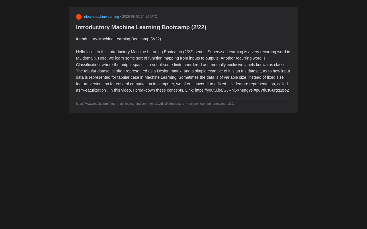
Supervised Learning: The Most Common Learning Paradigm in Machine Learning

In the field of machine learning, Supervised Learning is one of the most fundamental and widely applied paradigms. At its core, supervised learning is about learning a "function mapping from inputs to outputs."

To understand where supervised learning fits, you first need to understand the full landscape of machine learning paradigms. Machine learning is typically divided into three major paradigms: supervised learning, unsupervised learning, and reinforcement learning. The theoretical foundation of supervised learning can be traced back to the perceptron model proposed by Frank Rosenblatt in the 1950s. Among these paradigms, supervised learning is the most widely applied because it most closely resembles how humans learn—generalizing patterns from known examples. Unsupervised learning, on the other hand, doesn't rely on labels and attempts to discover inherent structure in data (such as clustering and dimensionality reduction); reinforcement learning learns decision-making strategies by interacting with an environment and receiving reward signals. Understanding the relationships between these three paradigms helps beginners choose the correct methodological framework when facing specific problems.

What Function Mapping Means

The goal of supervised learning is to find a function f such that, for a given input x, it can predict the corresponding output y. This process is called "supervised" because during the training phase, we provide the model with numerous sample pairs of known inputs and their corresponding outputs (i.e., labeled data). The model gradually "learns" the relationship between inputs and outputs by observing these samples.

From a deeper mathematical perspective, the process of finding this function mapping is essentially an optimization problem—adjusting model parameters by minimizing the difference between predicted values and true values (i.e., the Loss Function). This involves a key concept: Generalization, which refers to the model's performance on unseen new data. If a model merely "memorizes" the training data without being able to handle new data, Overfitting occurs; conversely, if the model is too simple to capture even the patterns in the training data, it's called Underfitting. This Bias-Variance Tradeoff is one of the most central theoretical challenges in supervised learning.

Here's an intuitive example: if we want a model to determine whether an email is spam, we first need to provide numerous email samples already labeled as "spam" or "normal." The model summarizes patterns from these samples and ultimately makes accurate judgments on new emails. This ability to "infer the unknown from the known" is the core value of supervised learning.

Classification: Supervised Learning Tasks with Discrete Output Spaces

Within supervised learning, Classification is a core task type. The defining characteristic of classification problems is that their output space is a set of finite, unordered, and mutually exclusive labels, called "Classes."

Three Key Characteristics of Classification Problems

Understanding classification requires grasping three key properties:

• Finite: The number of classes is definite and limited, for example, three classes: "cat, dog, bird."
• Unordered: There is no magnitude or sequential order between classes—"cat" is not "greater than" "dog."
• Mutually Exclusive: A sample can only belong to one class; it cannot simultaneously be both a "cat" and a "dog."

The Difference Between Classification and Regression

Classification stands in sharp contrast to another common supervised learning task—Regression. Regression outputs are continuous values (such as house prices or temperatures), while classification outputs are discrete class labels. Understanding this distinction is a prerequisite for choosing the correct algorithms and evaluation metrics.

Algorithm and Evaluation Ecosystem for Classification

Classification problems have spawned a rich ecosystem of algorithms. From the simplest K-Nearest Neighbors (KNN) and Naive Bayes, to Decision Trees, Support Vector Machines (SVM), and deep neural networks, different algorithms are suited for problems of different scales and complexities. Evaluation metrics for classification models also differ from regression: commonly used ones include Accuracy, Precision, Recall, F1 Score, and ROC-AUC curves. In class-imbalanced scenarios (such as fraud detection where normal transactions far outnumber fraudulent ones), accuracy alone can be misleading, and a more granular evaluation using a Confusion Matrix is needed. Choosing the right evaluation metric is often just as important as choosing the right algorithm.

Data Representation: The Design Matrix and the Iris Dataset

Machine learning cannot exist without data, and how data is represented in a computer directly affects algorithm design and performance. The Design Matrix is the standard way to organize tabular data.

Structure of the Design Matrix

For Tabular Data, we typically use a matrix to organize all samples: each row represents a sample (data point), and each column represents a Feature. This structured matrix is the design matrix. It organizes messy raw data into a neat form that computers can easily process, serving as the input starting point for the vast majority of machine learning algorithms.

The concept of the design matrix originates from linear regression theory in statistics, and is typically represented mathematically as X ∈ R^(n×d), where n is the number of samples and d is the feature dimension. This matrix-based data representation enables linear algebra operations to be efficiently applied to machine learning—matrix multiplication, eigenvalue decomposition, Singular Value Decomposition (SVD), and other operations form the computational core of many algorithms. The Tensor concept in modern deep learning frameworks (such as PyTorch and TensorFlow) is essentially a generalization of the design matrix to higher dimensions, making batch processing of complex data like images and sequences possible. Understanding the design matrix is not only foundational for traditional machine learning but also a bridge to deep learning.

Classic Example: The Iris Dataset

The Iris Dataset is the "Hello World" dataset for machine learning beginners, containing 150 iris flower samples. Each sample records four features—sepal length, sepal width, petal length, and petal width—with the goal of classifying them into one of three species.

This dataset was first used by British statistician Ronald Fisher in his 1936 paper to demonstrate the Linear Discriminant Analysis (LDA) method, making it nearly 90 years old. The dataset contains three species: Setosa, Versicolour, and Virginica. Setosa is linearly separable from the other two species in the feature space, while Versicolour and Virginica have some overlap, making it an ideal benchmark for testing the performance of different classification algorithms. In the scikit-learn library, it can be loaded directly with a single line of code: sklearn.datasets.load_iris(), and this convenience has further solidified its position as a standard teaching dataset.

The Iris dataset is widely used as a teaching example because its structure is simple and its dimensions are clear, perfectly demonstrating how tabular data is organized into a design matrix and the typical form of a classification problem. Through this dataset, beginners can quickly understand the correspondence between "feature vectors" and "labels."

Featurization: Converting Variable-Length Data into Fixed Vectors

Real-world data is not always neatly organized into fixed-length feature vectors. Data such as text, images, and audio often have variable sizes and structures. Featurization is the key step that solves this problem.

Why Featurization Is Indispensable

Traditional machine learning algorithms typically require inputs to be fixed-size feature vectors. However, a piece of text might have 10 words or 1000 words; an image might have varying resolutions. This variable-length data cannot be directly fed into many classical models.

The role of featurization is to convert this variable-sized raw data into fixed-size feature representations. Common featurization methods include:

• Text Featurization: Converting text into fixed-dimensional vectors using Bag-of-Words or TF-IDF. The Bag-of-Words model represents text as a vector of word occurrence counts from the vocabulary, while TF-IDF further considers term frequency and inverse document frequency, reducing the weight of common words (like "the" or "is") and increasing the weight of discriminative words.
• Image Featurization: Scaling images to a uniform size and extracting a fixed number of features. Traditional methods include hand-crafted feature descriptors such as HOG (Histogram of Oriented Gradients) and SIFT (Scale-Invariant Feature Transform).

Feature Engineering and the Deep Learning Paradigm Shift

Featurization is a core component of the broader practice of "Feature Engineering" in traditional machine learning. Before the rise of deep learning, feature engineering was considered the most time-consuming and domain-expertise-dependent phase of machine learning projects—there's a widely circulated saying in the industry: "Data and features determine the upper bound of machine learning, while models and algorithms merely approach that upper bound."

One of deep learning's revolutionary breakthroughs is automatically extracting features through End-to-End Learning, dramatically reducing the need for manual feature design. For example, Convolutional Neural Networks (CNNs) can automatically learn hierarchical feature representations of images, from low-level edges and textures to high-level object parts and semantic concepts; Transformer architectures can automatically learn contextual representations of text. However, in scenarios with limited data, constrained computational resources, or requirements for interpretability, carefully designed handcrafted features still hold irreplaceable value. For beginners, understanding the logic of manual featurization also helps in more deeply appreciating the significance of deep learning's "automatic feature extraction."

Featurization not only solves computational compatibility issues but also largely determines a model's final performance—good features are often more important than complex algorithms.

Summary and Learning Recommendations

This article has covered the four most essential concepts for beginners in machine learning:

1. Supervised Learning: Learning a function mapping from inputs to outputs through labeled data
2. Classification: A supervised learning task where outputs are finite, unordered, mutually exclusive class labels
3. Design Matrix: Organizing tabular data in the standard form of rows (samples) × columns (features)
4. Featurization: Converting variable-length raw data into fixed-size feature vectors

These four concepts have a clear progressive relationship: supervised learning defines the learning objective (learning input-to-output mappings), classification specifies a concrete output form (discrete classes), the design matrix prescribes how input data is organized (structured tables), and featurization addresses the practical challenge of how real-world data is transformed into the fixed format required by the design matrix.

For readers who want to systematically learn machine learning, it's recommended that after mastering these theoretical concepts, you get hands-on practice with classic cases like the Iris dataset by building a simple classification model using tools like scikit-learn. Specifically, you can try the following learning path: first train a model on the Iris dataset using scikit-learn's DecisionTreeClassifier or KNeighborsClassifier, observing how different hyperparameters affect classification results; then try practicing the featurization workflow on a text classification task (such as the 20 Newsgroups dataset). Combining theory with practice is the only way to truly internalize these abstract concepts. Interested readers can watch the original video for more detailed explanations.

Key Takeaways