LLM Inference Speed Formula: Memory Bandwidth Determines Your tokens/sec

Every week, someone in the community asks "which GPU should I buy to run LLMs locally," and the thread inevitably devolves into people listing whatever GPU they happen to own. But there's actually a calculable pattern behind all this—you only need two numbers from a spec sheet to predict your tokens/sec (tokens generated per second) with surprising accuracy. This article is compiled from a local LLM enthusiast's calculation logic repeatedly shared in Reddit comment sections.

It's Bandwidth That Determines LLM Inference Speed, Not Bus Width

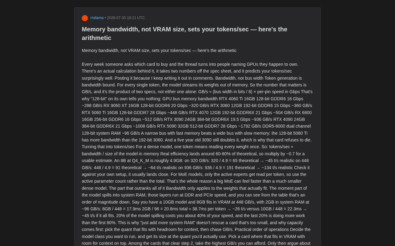
The token generation process of large models is bandwidth bound. In computer architecture, task bottlenecks are typically classified as either compute bound or bandwidth bound. The generation phase of LLM inference is bandwidth bound because when generating each token, the batch size is typically 1 (single-user local scenario), meaning each parameter is used for only one multiply-add operation, resulting in extremely low arithmetic intensity—far below the GPU's compute/bandwidth ratio (i.e., the knee point in the roofline model). This means the GPU's thousands of CUDA cores spend most of their time waiting for data to arrive from VRAM, with actual compute utilization potentially below 10%. For every token generated, the model must stream-read the entire set of weights from VRAM. Therefore, the number that truly determines speed is GB/s (memory bandwidth), which is the product of two specs rather than either one alone:

GB/s ≈ (bus width bits / 8) × per-pin data rate Gbps

This is why looking at "128-bit" alone is meaningless. The following comparison table illustrates this clearly:

GPU	Bus	Memory	Bandwidth
RTX 4060 Ti 16GB	128-bit	GDDR6 18 Gbps	~288 GB/s
RX 9060 XT 16GB	128-bit	GDDR6 20 Gbps	~320 GB/s
RTX 3060 12GB	192-bit	GDDR6 15 Gbps	~360 GB/s
RTX 5060 Ti 16GB	128-bit	GDDR7 28 Gbps	~448 GB/s
RTX 4070 12GB	192-bit	GDDR6X 21 Gbps	~504 GB/s
RX 6800 16GB	256-bit	GDDR6 16 Gbps	~512 GB/s
RTX 3090 24GB	384-bit	GDDR6X 19.5 Gbps	~936 GB/s
RTX 4090 24GB	384-bit	GDDR6X 21 Gbps	~1008 GB/s
RTX 5090 32GB	512-bit	GDDR7 28 Gbps	~1792 GB/s
DDR5-6000 Dual Channel	128-bit	System RAM	~96 GB/s

Understanding Memory Generations: From GDDR6 to GDDR7

The table features three different generations of memory technology, and understanding their differences helps decode the meaning behind the bandwidth numbers. GDDR6, introduced in 2018, typically offers per-pin rates of 14-18 Gbps using traditional PAM2 (two-level) signal encoding. GDDR6X, co-developed by NVIDIA and Micron, introduced PAM4 (four-level) signal modulation, transmitting 2 bits per clock cycle instead of 1, pushing per-pin rates to 19-24 Gbps. GDDR7 is the latest standard officially released by JEDEC in 2024, employing PAM3 (three-level) encoding with per-pin rates reaching 28-36 Gbps, while also adopting a dual-channel architecture for improved bandwidth efficiency. This explains why with the same 128-bit bus width, the 5060 Ti with GDDR7 can exceed the 4060 Ti with GDDR6 by over 55% in bandwidth.

Several counter-intuitive conclusions emerge from the table: a narrow bus with fast memory can beat a wide bus with slow memory. The 128-bit 5060 Ti (448 GB/s) actually has higher bandwidth than the 192-bit 3060 (360 GB/s). And the five-year-old 3090 still delivers about 936 GB/s—nearly double that of mainstream new cards—which is why this card refuses to retire in the local inference community.

Converting Memory Bandwidth to tokens/sec

For a dense model, generating one token means reading all weights once. So you can estimate directly:

tokens/sec ≈ bandwidth / model size in VRAM

Real-world efficiency typically falls between 60%–80% of the theoretical value, so using a coefficient of approximately 0.7 gives a usable estimate. Taking an 8B parameter model with Q4_K_M quantization at roughly 4.9GB as an example:

About Q4_K_M Quantization

Q4_K_M is a widely used mixed-precision quantization format in the llama.cpp ecosystem. "Q4" indicates the main weights are quantized to 4-bit integers, "K" stands for k-quant method (a block quantization strategy where weights within each block share scaling factors and minimum values), and "M" means Medium precision tier. In the k-quant system, different layers are assigned different precision levels based on their sensitivity to output quality: key matrices in attention layers may retain 6-bit precision, while most feed-forward network weights are compressed to 4-bit. An 8B parameter model that's approximately 16GB in original FP16 format typically shrinks to 4.5-5.0GB after Q4_K_M quantization, while perplexity increases only about 0.5-1.5% compared to FP16—making it the community's consensus sweet spot for balancing quality and size.

Back to the calculation examples:

• 320 GB/s: 320 / 4.9 ≈ 65 theoretical → ~45 t/s actual
• 448 GB/s: 448 / 4.9 ≈ 91 theoretical → ~64 t/s actual
• 936 GB/s: 936 / 4.9 ≈ 191 theoretical → ~134 t/s actual

You can benchmark your own machine and compare—results typically track very closely to this estimate.

Why MoE Models Run Faster at Inference

For MoE (Mixture of Experts) models, each token only reads the activated subset of expert weights, so you should use the active parameter count rather than total parameters in the formula.

The core idea of MoE is to split the feed-forward network (FFN) layers into multiple parallel "expert" sub-networks, where each token selectively activates only a few experts through a gating network (router/gate). For example, Mixtral 8x7B has approximately 46.7B total parameters, but each token activates only 2 out of 8 experts, with actual active parameters around 12.9B. This means the model requires more VRAM to store all expert weights, but the amount of data actually read from VRAM per step is dramatically reduced. In bandwidth-bound inference scenarios, this directly translates to higher tokens/sec. DeepSeek-V3, Qwen's MoE variants, and others all employ similar designs—this is precisely why a massive MoE model can actually feel faster than a much smaller dense model.

The Performance Cost of Spilling to System Memory

The bandwidth premise assumes that these weights actually fit in VRAM. Once any part of the model spills to system memory, those layers run at DDR and PCIe speeds—as the table shows, this is an order-of-magnitude drop (96 GB/s versus hundreds of GB/s).

The Secondary PCIe Bottleneck

It's worth noting that even if your system memory bandwidth is nominally 96 GB/s (DDR5-6000 dual channel), the actual rate at which the GPU can fetch this data is further constrained by the PCIe bus as a secondary bottleneck. PCIe 4.0 x16 has a theoretical unidirectional bandwidth of 32 GB/s, PCIe 5.0 x16 offers 64 GB/s, but actual effective bandwidth is further reduced by protocol overhead. In frameworks like llama.cpp, the model is split by layer (layer offloading)—some layers execute on GPU, others on CPU, with intermediate results transferred via PCIe, each cross-bus transfer introducing additional latency. This also explains why the performance degradation from "partial offloading" is often non-linear.

Here's an example: suppose you have a 10GB model where 8GB fits in 448 GB/s VRAM, and the remaining 2GB falls to ~96 GB/s system memory:

8GB / 448 = 17.9ms
2GB / 96  = 20.8ms
Total ≈ 38.7ms/token → ~26 t/s

Whereas if everything fits in VRAM:

10GB / 448 = 22.3ms → ~45 t/s

The conclusion is stark: just 20% of the model spilling causes roughly 40% speed loss. In other words, that last 20% of weights drags performance more than the first 80% combined. This explains why "just adding more system RAM" can't save a card with too little VRAM, and why VRAM capacity takes priority over bandwidth.

GPU Selection Decision Order for Local LLM Deployment

The author provides a clear operational hierarchy worth referencing for anyone doing local deployment:

1. First, determine your model tier: Decide which class of models you want to run, and confirm the actual size based on the quantization format you'll use.
2. Pick a card that fits the model: Ensure the model fits in VRAM, with headroom left for context.
3. Among cards that fit, choose the highest bandwidth: Within budget, pursue the highest GB/s.
4. Worry about ecosystem last: CUDA vs ROCm vs Vulkan does affect deployment convenience, but it determines hassle factor, not performance ceiling.

Why You Need to Reserve VRAM for Context

The "leave headroom for context" mentioned in step two deserves special explanation. Beyond model weights themselves, the inference process also requires VRAM allocation for KV Cache (key-value cache). KV Cache stores the key and value vectors from every attention layer for the generated sequence so far, with its size proportional to context length, number of layers, and number of attention heads. For example, a 32-layer, 32-head, dimension-4096 model at FP16 precision uses approximately 256MB of VRAM per 1024 tokens of KV Cache. When the context window expands to 32K or even 128K tokens, KV Cache can consume several GB of VRAM. Therefore, when selecting a card, you can't just calculate "the model barely fits"—you must reserve sufficient space for KV Cache, otherwise during long conversations you'll either be forced to truncate context or trigger spillover to system memory causing severe slowdowns.

Final Thoughts

This "two numbers to calculate tokens/sec" methodology essentially pulls local LLM hardware selection out of mysticism and back into engineering calculation. The core logic condenses to one sentence: first check whether VRAM capacity can fit the model, then look at how fast the bandwidth is, and leave ecosystem concerns for last.

It should be noted that the ~0.7 efficiency coefficient is an empirical value the author summarized from their own multiple machines, not a precise constant. Different inference frameworks (llama.cpp, vLLM, ExLlamaV2, etc.), quantization methods (GGUF, GPTQ, AWQ, EXL2, etc.), and batching strategies will all cause this coefficient to fluctuate. Additionally, during the prefill phase (batch computation when processing the input prompt), the task may become compute bound, where GPU compute power (TFLOPS) also comes into play—but for the generation speed (decode phase) that local users care most about, bandwidth remains the sole determining factor.

If you have benchmark data on hand, try validating it against the formula—this is the best thing about this method: it doesn't require you to trust anyone's recommendation. Your own machine is the ultimate test.