LogCDM: How a Small Model Achieves Interpretable Log Anomaly Detection via Behavior Graph Drift

LogCDM achieves millisecond log anomaly detection on CPU with an 8M-parameter model, F1 approaching large models.
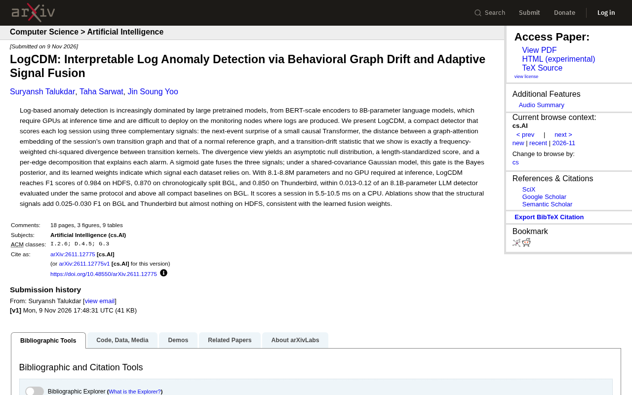
LogCDM is a lightweight log anomaly detection method that scores a single session in 5.5–10.5 ms on CPU with only 8.1–8.8M parameters, its F1 differing by just 0.013–0.12 from LLM detectors three orders of magnitude larger. It fuses next-event surprise, graph-attention embedding distance, and transition-drift statistics via a sigmoid gate equivalent to a Bayesian posterior. Transition drift is proven to be a frequency-weighted chi-square divergence, yielding an asymptotic null distribution, length-normalized scores, and per-edge alert explanations. On HDFS, BGL, and Thunderbird, LogCDM performs strongly; structural signals add 0.025–0.030 F1 on BGL and Thunderbird but contribute almost nothing on HDFS, consistent with gate weights. The method approaches large-model accuracy while greatly reducing inference cost and embedding interpretability, offering a practical solution for resource-constrained log monitoring.
Log anomaly detection is being swept by large models — from BERT-level encoders to 8-billion-parameter language models, inference requires GPUs, making deployment on the monitoring nodes that generate logs nearly unthinkable. LogCDM proposes a counterintuitive path: a small detector with only 8.1–8.8M parameters that scores a single session in 5.5–10.5 milliseconds on CPU, with F1 scores approaching LLMs three orders of magnitude larger.
Three Signals, One Gate: LogCDM's Fusion Logic
LogCDM's core design routes three complementary signals through a sigmoid gate for fusion. The first is "next-event surprise" from a small causal Transformer, capturing sequence-level anomalies; the second is the distance between the graph-attention embedding of the session's own transition graph and a normal reference graph, characterizing structural deviation; the third is a transition-drift statistic — the paper proves it is exactly the frequency-weighted chi-square divergence between transition kernels.
This divergence perspective is no mathematical ornament. It directly yields three practical products: an asymptotic null distribution, giving threshold setting a statistical basis; a length-normalized score, eliminating bias from session length; and per-edge decomposition, allowing every alert to be traced back to a specific transition edge. This last point is the key to interpretability — operators see not an isolated anomaly score, but "which state transition deviated from the normal pattern."
Under a shared-covariance Gaussian model, this sigmoid gate is equivalent to a Bayesian posterior, and the learned weights directly reflect which signal each dataset relies on. This explains why structural signals contribute markedly differently across datasets.
Transition kernels and chi-square divergence: In log anomaly detection, a session can be viewed as a Markov chain whose transition kernel defines the probability distribution of moving from one event type to another. Normal and anomalous sessions often differ in their transition kernels. Frequency-weighted chi-square divergence is a statistic measuring the difference between two probability distributions; it weights each transition edge by frequency and computes the deviation of observed transitions from expected ones. The paper proves the transition-drift statistic is exactly an instance of this divergence, giving it favorable statistical properties: under normal data it asymptotically follows a chi-square distribution, so significance thresholds can be set directly; moreover, the divergence decomposes onto each transition edge, enabling fine-grained anomaly localization. This statistical-divergence approach is lighter and more interpretable than learned methods.
Graph-attention embeddings and distance to a reference graph: A graph attention network (GAT) aggregates neighbor information via attention to produce an embedding for each node. In the log setting, feeding a session's transition graph into a GAT yields a graph embedding that encodes the session's structural pattern. The normal reference graph is obtained by averaging or clustering the graph embeddings of normal sessions in the training set, representing the normal structural prototype. The Euclidean or cosine distance between an anomalous session's graph embedding and the reference embedding reflects structural deviation: the larger the distance, the more likely it is anomalous. This method captures anomalies in event co-occurrence and transition relationships, but depends on the quality of the reference graph and the coverage of normal samples.
Performance: The Gap to Large Models Is Measured in Tenths of a Decimal
Under a unified evaluation protocol, LogCDM achieves an F1 of 0.984 on HDFS, 0.870 on chronologically split BGL, and 0.850 on Thunderbird. For reference, an 8.1B-parameter LLM detector under the same protocol differs from LogCDM by only 0.013–0.12. On BGL, LogCDM surpasses all compact baselines.
The inference-cost comparison is stark: LogCDM takes 5.5–10.5 milliseconds per session on CPU, with no GPU needed. For scenarios requiring deployment close to where logs are generated, this difference determines whether a solution is feasible at all.
Ablation experiments reveal the details of signal fusion: the structural signal yields an F1 gain of 0.025–0.030 on BGL and Thunderbird, but contributes almost nothing on HDFS. This is consistent with the fusion weights learned by the gate — HDFS anomaly patterns manifest more in the event sequences themselves than in transition-graph structure. In other words, the fusion weights serve not only prediction but also as a diagnostic tool for dataset characteristics.
F1 score and evaluation protocol: The F1 score is the harmonic mean of precision and recall, commonly used for imbalanced classification tasks. In log anomaly detection, anomalous samples are scarce, and F1 comprehensively evaluates a detector's ability to identify anomalies. The evaluation protocol refers to the data split method (e.g., random or chronological), preprocessing steps, and metric computation rules. Chronological splits are closer to real deployment but may introduce distribution drift, leading to lower performance than random splits. HDFS, BGL, and Thunderbird are commonly used log datasets from a distributed file system, a supercomputer, and a mail server, respectively, with varying anomaly patterns and scales. A unified evaluation protocol ensures fair comparison across methods.
Rebalancing Interpretability and Deployment Trade-offs
Log anomaly detection has long faced a trilemma: detection accuracy, inference cost, and interpretability are hard to achieve simultaneously. Large models push the accuracy ceiling higher but shift the cost onto infrastructure; traditional statistical methods are lightweight and interpretable but limited in accuracy. LogCDM's entry point is to embed interpretability into the detection mechanism itself rather than attaching an explanation module after the fact.
Per-edge decomposition makes alerts actionable: the system not only reports "this session is anomalous" but also identifies which specific transition's drift triggered the alert. The chi-square divergence statistical framework provides an asymptotic null distribution, freeing threshold selection from empirical tuning. These properties have practical value for production environments requiring auditing and root-cause localization.
Of course, the paper leaves open questions. The failure of the structural signal on HDFS shows that graph-drift methods carry assumptions about the graph-structure sensitivity of logs; how to fairly compare the chronologically split BGL result (0.870) with the conventional random-split reports still needs community consensus. In addition, how the reference graph is constructed and the coverage of normal samples both affect the quality of the distance signal.
LogCDM's value lies not in rejecting the large-model path but in delineating a neglected engineering boundary: when deployment sits close to the log source and when explanation needs are as important as detection needs, a carefully designed compact detector paired with a statistically interpretable fusion mechanism can approach large-model accuracy while being orders of magnitude cheaper. For operations systems with massive log volumes and resource-constrained monitoring nodes, this is an option worth serious evaluation.
Asymptotic null distribution and threshold setting: The asymptotic null distribution refers to the distribution a statistic approaches as sample size grows under normal data. For chi-square divergence, under the null hypothesis (no anomaly), the statistic asymptotically follows a chi-square distribution whose degrees of freedom relate to the number of transition edges. Using this property, thresholds can be set to control the false-positive rate at a given level (e.g., p-value below 0.05), avoiding reliance on empirical tuning. The length-normalized score normalizes the statistic by session length, eliminating the effect of session length so that sessions of different lengths are comparable. Per-edge decomposition splits the total divergence into each transition edge's contribution, thereby localizing anomalous transitions. Together these properties enhance the statistical rigor and interpretability of detection.
One-line Summary
LogCDM uses an 8M-parameter small model to achieve millisecond-level log anomaly detection on CPU, with F1 approaching large models.
Paragraph Summary
LogCDM proposes a lightweight log anomaly detection method that scores a single session in 5.5–10.5 ms on CPU with only 8.1–8.8M parameters, its F1 differing by just 0.013–0.12 from LLM detectors three orders of magnitude larger. At its core, three signals — next-event surprise, graph-attention embedding distance, and transition-drift statistics — are fused via a sigmoid gate that is equivalent to a Bayesian posterior under a shared-covariance Gaussian model. Transition drift is proven to be a frequency-weighted chi-square divergence, yielding an asymptotic null distribution, length-normalized scores, and per-edge alert explanations. On HDFS, BGL, and Thunderbird, LogCDM performs strongly; the structural signal adds 0.025–0.030 F1 on BGL and Thunderbird but contributes almost nothing on HDFS, consistent with the gate weights. The method approaches large-model accuracy while greatly reducing inference cost and embedding interpretability, offering a practical solution for resource-constrained log monitoring scenarios.
Related articles

Gemini 4 Neon Opens Paid API: Million-Token Long Tasks and Local LLM Benchmarks
Gemini 4 Neon opens its paid API with 1M-token context at $3/$15 per million tokens; OpenAI live dictation drops the 10-minute limit; local LLM tests show order-of-magnitude speed gaps; GitHub Skills rankings update.

Gemini 4 Neon Hands-On: Crushing Claude on Value, But Two Pitfalls
Gemini 4 Neon hands-on: ranks 2nd on KingBench 4 at 37.9/60 across six projects, doing for $20.36 what cost Fable 5.2 $222 — but container escapes and dead-API coding expose blind spots.

Anthropic IPO: The AI Gamble Behind a $1.33 Trillion Valuation
Anthropic launches its IPO at a $1.33T fully diluted valuation. Of its $104B nine-month GAAP loss, $94.3B is non-cash. Morningstar sees $92; Michael Burry flags $900B compute risk.