MoE (Mixture of Experts) Deep Dive: Principles, Formulas, and Implementation
MoE splits large FFNs into specialized experts with sparse activation—more capacity, less compute
MoE (Mixture of Experts) resolves the dense model dilemma by splitting large FFNs into multiple small experts, activating only the most relevant ones per token. This sparse activation approach increases total model capacity while reducing per-pass computation. Key innovations include fine-grained expert splitting, shared experts for common capabilities, and load balancing losses to prevent expert collapse. Understanding MoE reveals how modern large models maximize knowledge capacity within compute budgets.
The Dilemma of Dense Models
In traditional Transformer architectures, each layer primarily consists of two components: the Attention module, which computes relationships between tokens, and the Feed-Forward Network (FFN) module, which independently applies non-linear transformations to each token's features. Since Google's "Attention Is All You Need" paper in 2017, the Transformer architecture has become the foundation of modern large language models. Its FFN typically uses a two-layer linear transformation with an activation function (like ReLU or SiLU) sandwiched between, responsible for independent local feature extraction and non-linear transformation of each token after attention captures global relationships.
To improve large model performance, the most direct approach is to follow Scaling Laws—continuously increasing parameter count. Scaling Laws, systematically articulated by OpenAI in 2020, revealed near power-law relationships between model performance and parameter count, data volume, and compute, driving the birth of massive models like GPT-3 (175B parameters) and PaLM (540B parameters). However, these laws don't specify how to scale efficiently—simply expanding dense models means training and inference compute requirements balloon in lockstep, causing deployment costs to skyrocket. For FFNs, the most common expansion approach is widening the intermediate dimension, say from D to 2D or 4D. Parameter count increases, and performance typically improves. But there's a fundamental contradiction: every token must pass through the entire set of weights. Taking "follow Bilibili to learn about large models" as an example, every token goes through the same weight matrices W1 and W2. The wider the FFN, the more computation scales linearly.
This is the dense model dilemma: it cannot balance "more parameters" with "less computation"—the two are fundamentally at odds. MoE (Mixture of Experts) was born to resolve this contradiction.
MoE Core Idea: Sparse Activation
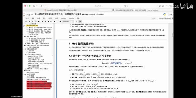
MoE's approach is straightforward: split one large FFN into N small FFNs, call each small FFN an "expert," then use a router/gating network to decide which experts to activate each time.
MoE is not a new invention of the large model era. As early as 1991, Jacobs et al. proposed the prototype of mixture of experts models in neural networks; in 2017, Google Brain's Shazeer et al. introduced it to deep learning, demonstrating for the first time the feasibility of scaling MoE to large-scale language models; subsequent work like Switch Transformer (2021) further refined MoE implementation in Transformer architectures, laying the engineering foundation for modern MoE large models like DeepSeek.
For example: expand the original FFN by 4x, then split it into 8 small experts. When a token comes in, instead of activating all 8, use the router network to select only the few most relevant to the current task for computation.
This design simultaneously achieves two seemingly contradictory goals:
- Larger total model parameters: increased capacity to hold more knowledge
- Less computation per forward pass: only activate the most relevant experts each time, others don't participate in computation
With N experts, selecting only Top-K each time (typically K=1 or 2), the actual computation ratio is only 1/8 or 2/16. K=2 is currently the most common choice in practice, striking a good balance between computational efficiency and model quality—DeepSeek-MoE, Mixtral 8x7B, and others all use this setting. While total parameters increase, FLOPs per forward pass actually decrease. This is MoE's sparse activation philosophy.
From "Generalist" to "Domain Expert"
A large FFN can be understood as a "generalist"—knows a bit about everything. Each small FFN after splitting focuses on a specific domain. When input is about sports, activate the sports expert; history topics activate the history expert; finance topics activate the finance expert.
Activating finance and entertainment experts for history questions is meaningless—they have no accumulated knowledge in that domain. This targeted activation is the root of MoE's efficiency.
Mathematical Formula Derivation
Expert Network Definition
Each expert is essentially a two-layer FFN: linear upscaling → non-linear activation → linear downscaling. Assuming D=4096, the original dense FFN upscales to 16384 (4x) then back down to 4096, with computation roughly 2×D×4D = 8D².
After splitting, each expert's intermediate dimension is only one-quarter of the original, with single expert computation of 2×D×D = 2D². The total parameter-equivalent computation for 8 experts is 8×2D² = 16D², twice the original dense model.
The key point: if only 2 experts are activated each time, the actual computation is only 2×2D² = 4D², half of the original dense FFN (8D²). Total capacity doubles while single-pass computation halves.
Router Network Computation
The Router network decides which experts each token should consult. It's a lightweight linear layer that maps tokens to N-dimensional logits, then applies Softmax to get selection probabilities for each expert:
g = Softmax(Wg · x)
Higher probability g means the router considers that expert more suitable for processing the current token. In practice, only Top-K experts are selected, not all of them (otherwise it degrades to a dense model). Worth noting is that different experts can be distributed across different GPUs to achieve "expert parallelism," but routing tokens to remote GPUs introduces communication overhead, making MoE's actual training efficiency more complex than theoretical analysis suggests.
Weighted Sum Output
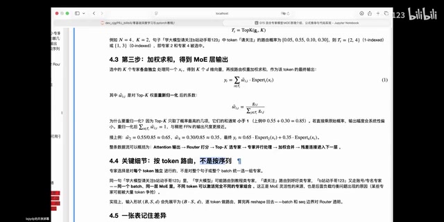
After selecting K experts, each independently processes the input token, yielding K output vectors. Finally, a weighted sum is computed using normalized selection probabilities. For example, if experts 2 and 4 are selected with probabilities 0.55 and 0.3 respectively, normalization is first needed (divide by 0.85) to ensure weights sum to 1, then the two output vectors are weighted and summed. This embodies an ensemble thinking.
Evolution of Mainstream MoE Architectures
Fine-Grained Expert Splitting
Traditional MoE has a problem: expert division is too coarse. The FFN itself is already huge; if split into only 2 or 4 experts, each expert is still forced to learn large amounts of unrelated knowledge, failing to maximize the expert mechanism.
DeepSeek's first innovation is fine-grained expert splitting—increasing expert count from N to 2N or even more. The theoretical basis is: when expert count is small, each expert must cover too broad a semantic space, leading to high knowledge overlap between experts and insufficient specialization. By splitting the same total parameter count into more, smaller experts, each expert only needs to cover a finer-grained semantic subspace, and the router network has much larger combinatorial space when selecting K experts—expanding from C(8,2)=28 combinations to C(64,6)≈74.6 million, theoretically enabling more precise matching of processing needs for different tokens. It's like a hospital shouldn't have just two doctors for internal and external medicine, but should subdivide into gastroenterology, hepatobiliary, ENT, etc.
Shared Experts
The second innovation is Shared Experts. Research found that multiple routed experts would independently learn nearly identical weights, forming "expert collapse"—this redundancy not only wastes parameters but also exacerbates load imbalance. All experts may need to learn some general foundational capabilities, like grammar rules and common collocations. Splitting these general capabilities makes little sense and causes redundant computation.
Therefore, general capabilities can be extracted as shared experts, activated every time without participating in Top-K selection. This architecturally resembles the intuition of "skip connections handling general features" in residual networks—shared experts handle basic transformations needed by all tokens, while routed experts focus on differentiated domain knowledge. Like a hospital blood draw center—rather than equipping every department with blood draw facilities, centralize it at a common service desk for unified access. DeepSeek-V2 adopted a configuration of 1 shared expert plus multiple routed experts, achieving better results in practice than pure routed MoE. Fine-grained experts + shared experts constitute the current mainstream MoE model architectural paradigm.
Three Key Parameter Concepts Clarified
Understanding MoE requires distinguishing three parameter concepts:
- Total parameters: All N experts' parameters must be stored in VRAM or disk, regardless of how many are activated. With D=4096 and 8 experts, total parameters can reach 536M
- Activated parameters: The K experts selected by routing participate in computation, determining actual computational overhead, approximately 134M
- VRAM occupation: Processing requires KV Cache plus all experts' resident parameters. Sparse activation doesn't reduce VRAM occupation; VRAM mainly depends on total parameters
There's an important deployment reality here: during inference, all expert weights must be simultaneously loaded into GPU VRAM; otherwise, each token's routing would require frequent disk IO, making inference latency unacceptable. Taking Mixtral 8x7B as an example, its total parameters are about 46.7B, but activated parameters per forward pass are only about 12.9B—inference speed approaches a 13B dense model, yet requires VRAM for storing 46.7B parameters (about 90GB fp16). This is MoE's core tradeoff of "large capacity, low compute": activation is only one-quarter of total parameters, but VRAM requirements don't get discounted.
Load Balancing: MoE's Core Challenge
In actual training, MoE encounters load imbalance problems. Suppose there are 64 experts with 8 activated each time, but during training tokens particularly favor one or two experts while the rest are almost never activated.
This causes two problems: first, idle experts waste VRAM; second, popular experts are repeatedly overloaded, slowing processing speed. It's like a few doctors being mobbed by hundreds of patients while other doctors sit idle.
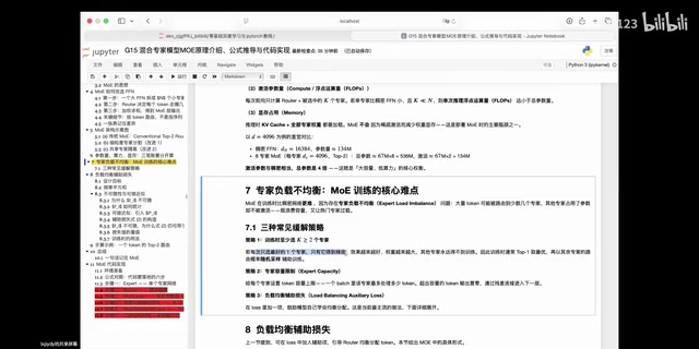
Three strategies typically address this:
- Select at least K≥2 experts during training: Sample sub-optimal experts with certain probability, letting them participate in training iterations
- Expert capacity limits: Set token processing caps for each expert, like "appointment slots," after which tokens must turn to other experts when full
- Load balancing auxiliary loss: Apply constraints in the loss function—this is the most critical measure
Load Balancing Loss Derivation
The balancing goal is to make each expert's selection probability Fi as close as possible to the average 1/N. Use the sum of squares of all expert frequencies to measure distribution balance:
L = Σ Fi²
By the Cauchy-Schwarz inequality, this loss is minimized if and only if all Fi = 1/N. With extreme imbalance (F1=1, F2=0) the sum of squares is 1; with perfect balance (F1=F2=0.5) the sum of squares is 0.5—the more concentrated the distribution, the larger the loss.
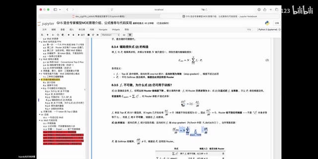
But this loss has a critical problem: it's non-differentiable. The root cause is the discrete nature of Top-K operations: Top-K selection is essentially threshold truncation after sorting, with gradients with respect to routing weights nearly zero everywhere at the boundary between selected and unselected, unable to pass effective learning signals to the router network. Forcing differentiation yields gradient identically 0, and the router network receives no useful signal.
The solution is introducing a differentiable proxy quantity Pi—the batch-averaged Softmax probability of tokens for each expert. Replace one Fi in Fi² with Pi:
L = N · Σ (Fi · Pi)
Where Fi is the post-hoc statistics of actual token selection (treated as constant, no gradient during backprop), and Pi is the differentiable soft probability (carrying gradient). This product form mathematically ensures: when fi is biased high, gradients push pi lower, achieving balance. The final total loss is:
Loss_total = LM_loss + α · L_balance
α requires careful tuning: too large causes "absolute egalitarianism," damaging primary task performance; too small renders balancing constraints basically ineffective. Worth mentioning, DeepSeek further introduced expert-level bias term dynamic adjustment on this basis, exploring directions for achieving good balancing effects without auxiliary loss.
Code Implementation Essentials
Complete MoE implementation involves several modules:
- Single expert network: Two Linear layers plus activation function—input X is first upscaled, activated, then downscaled
- Router network: Linear projection on input X followed by Softmax, take Top-K and normalize to ensure each row's weights sum to 1
- MoE layer: Create N independent experts (assembled with ModuleList) plus router network, through nested loops—outer loop iterates over each token, inner loop iterates over K experts selected by that token, processes and accumulates weighted by weights
- Load balancing loss: Calculate post-hoc statistical frequency F and differentiable average Softmax probability P separately, then sum by formula
N · Σ(F·P) - Shared expert: Doesn't participate in routing selection, fully activated every time, added to routed expert results
Summary
MoE is a milestone architectural innovation in large model development. Scaling Laws revealed the pattern that "expanding parameters improves performance," but the computational explosion from dense scaling became a practical bottleneck. MoE splits large FFNs into multiple small experts with sparse activation, increasing model capacity while actually reducing per-pass computation—this approach evolved from the 1991 theoretical prototype, refined through engineering practices like Switch Transformer, and ultimately matured in models like DeepSeek-V2/V3. A series of engineering improvements including fine-grained splitting, shared experts, and load balancing loss have brought this architecture to true maturity, making it a core component of mainstream large models represented by DeepSeek. Understanding MoE is essentially understanding the deeper question of "how to maximize model knowledge capacity within limited compute budgets."
Key Takeaways
Related articles

Climate Resilience Assessment of Global Megacities: Who Stands Strongest Against Disaster?
An in-depth look at climate resilience across global megacities, comparing how developed and developing cities handle extreme weather, sea-level rise, and other climate disasters.
Porting NES to CUDA: 20x Speedup in Mario Reinforcement Learning Training
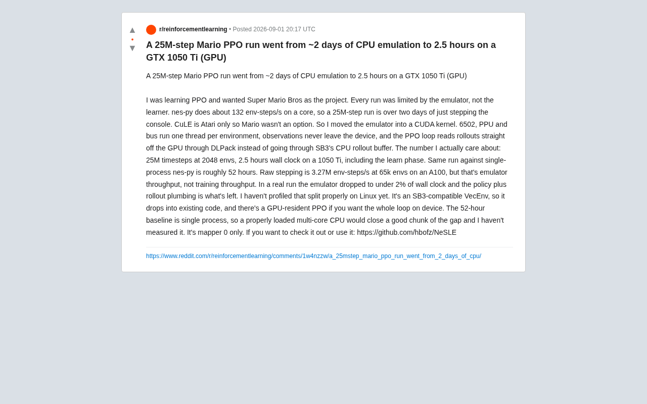
Developer ports complete NES emulator to CUDA kernels, achieving GPU parallel execution of 2048 Mario environments. On GTX 1050 Ti, 25M-step PPO training drops from 52 hours to 2.5 hours—nearly 20x faster. Deep dive into NeSLE's technical architecture and performance data.
Chinese Open-Source LLMs Dominate Hugging Face: The Flash Lightweight Era
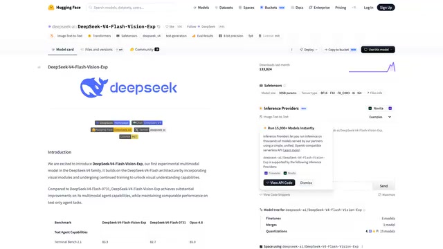
Five of Hugging Face's top six trending models are Chinese. DeepSeek V4 Flash Vision tops the chart. Why Flash lightweight versions are more popular than flagships, featuring Qwen, GLM, and other locally deployable open-source models. Analysis of MoE sparsification trends and selection advice.