PPO Parallel Robot Training: How to Scale to Thousands of Agents?

In real-world reinforcement learning (RL) applications, training speed is often a bigger headache than algorithm design. A developer on Reddit ran into exactly this problem: using ML-Agents and Unity to train a quadruped robot, everything worked well with 10 parallel environments—but it took 3 hours to see results. When he tried scaling the number of parallel robots to 100 or even 1000, the training curve collapsed instead. His hardware could theoretically support 10,000 robots training simultaneously, but he had no idea how to adjust the hyperparameters.

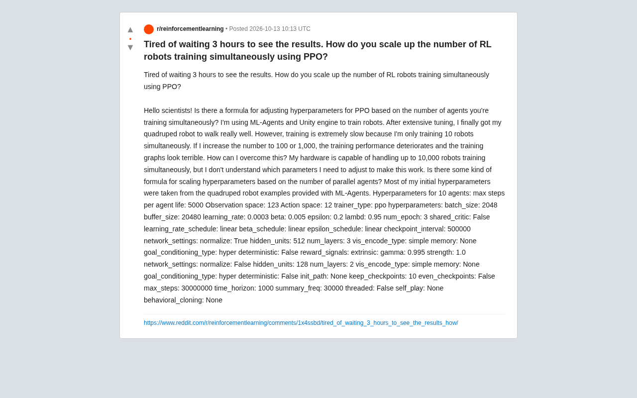
This problem is extremely typical in robot simulation training. The core tension is this: increasing the number of parallel environments does not equal simply scaling up batch_size or buffer_size proportionally. PPO's stability depends on the correlation of experience data and the consistency of policy update pacing. When the number of environments surges, the variance of gradient estimates, the sparsity of reward signals, and the frequency of network updates all undergo qualitative changes.

Why Does Parallel Environment Scaling Cause Performance Collapse?

PPO's Data Collection Mechanism Breaks Down

PPO is an on-policy algorithm, meaning the data used for each update must come from the current policy. In ML-Agents, buffer_size determines how much experience is collected before each update. With only 10 environments, each environment contributes relatively complete trajectories; when the number of environments expands to 1000, the same buffer_size means each environment only contributes extremely short fragments. This leads to two problems: first, the bias in advantage function estimation increases because trajectories are truncated; second, the value network struggles to learn long-range dependencies because each environment's temporal horizon is diluted.

On the relationship between on-policy and buffer_size: In ML-Agents, buffer_size corresponds to the total number of experience steps PPO collects between two policy updates (roughly equal to num_envs × time_horizon). Since PPO is an on-policy algorithm, this batch of data is discarded after completing num_epoch gradient updates, and the next round must resample with the latest policy. Therefore, a larger buffer doesn't mean data can be reused—it means a single update consumes more samples. When the number of environments scales from 10 to 1000, if buffer_size remains unchanged, the trajectory length allocated to each environment gets compressed to 1/100 of the original. In extreme cases, a single environment might only contribute a few time steps, and trajectories are severely truncated in time. This directly undermines the advantage function (GAE) estimation of returns—GAE relies on accumulating consecutive temporal-difference residuals, and shorter trajectories mean larger bootstrap bias. Meanwhile, the value network also needs a sufficiently long temporal horizon to learn the correspondence between state values and long-term returns. Therefore, the essential purpose of scaling buffer_size alongside parallel count is to ensure each environment still contributes a usable stretch of continuous trajectory—not simply to have "more data."

Implicit Coupling Among Hyperparameters

In the original configuration, time_horizon: 1000 and max_steps: 5000 were designed for a small number of agents. When the parallel count increases, each agent actually experiences far fewer time steps per update round. If you continue using summary_freq: 30000, you'll see extremely unstable reward curves in early training. More critically, the combination of learning_rate: 0.0003 and num_epoch: 3 causes each update to change the policy too drastically when many environments run in parallel—because the total sample size surges, the effective step size of gradient updates is amplified under the same learning rate.

On the coupling of learning_rate, batch_size, and update magnitude in PPO: PPO's stability comes from the "small step update" constraint, whose mathematical form is jointly determined by the clip objective and the learning rate. The effective step size of a gradient update can be roughly viewed as learning_rate × (variance of the gradient estimate). When batch_size scales linearly with the number of environments, the variance of the gradient estimate decreases at approximately 1/batch_size—meaning the gradient direction is more accurate, but the per-step magnitude doesn't automatically change. However, under a fixed learning_rate, since each update round uses more samples while the number of epochs stays the same, the total displacement pushing the policy toward a new distribution within a single iteration may actually increase, manifesting as violent oscillation or even collapse of rewards in early training. This is precisely why num_epoch: 3 becomes dangerous with massive parallel environments: the same batch of data gets used 3 times, and if that batch's size has surged, each epoch pushes the policy further. Common mitigation strategies in practice include reducing the learning rate by a sqrt ratio, enabling linear learning rate decay, or using gradient clipping with adaptive optimizers (like Adam) to keep the per-step update magnitude within a range matching the policy distribution change.

Empirical Formulas and Strategies for Hyperparameter Scaling

Although there's no officially published precise formula, the community has distilled some scaling principles from practice. The core idea is: maintain the balance between the effective sample size per gradient update and the policy update magnitude.

Linear Scaling of batch_size and buffer_size

The most direct rule of thumb: when the number of parallel environments increases from N to M, batch_size should increase at least linearly by a factor of M/N. For example, scaling from 10 environments to 1000, batch_size should increase from 2048 to approximately 204800. Meanwhile buffer_size should remain 5-10× batch_size to keep PPO's clip mechanism effective. But note that an excessively large batch_size reduces sample efficiency, so it's recommended to scale in stages: first to 100 environments, then gradually to 500, 1000.

Adjusting Learning Rate and Update Epochs

Learning rate scaling is controversial. One conservative approach is to keep the learning rate unchanged but increase num_epoch or use a larger batch_size to stabilize gradients. Another approach is square-root scaling: multiply the learning rate by sqrt(M/N). For example, from 10 to 1000, the learning rate would be adjusted to 0.0003 * sqrt(100) = 0.003. But this may be too aggressive in ML-Agents—it's advisable to start with 1.5-2× and experiment.

Redesigning Temporal Horizon and Network Architecture

time_horizon should be appropriately reduced, because with many environments running in parallel, each environment doesn't need to collect overly long trajectories. Try reducing from 1000 to 200-500. At the same time, hidden_units: 512 and num_layers: 3 may be too small for 1000 parallel environments—the policy network needs stronger representational capacity to distinguish state distributions across different environments. Consider increasing to 1024 units or adding another layer.

On the relationship between time_horizon, parallel environments, and long-range dependencies: time_horizon in ML-Agents defines the maximum number of consecutive steps each agent samples between two policy updates—it determines the upper bound on a single trajectory's length. The more parallel environments, the more total steps agents interact with the environment per unit of real time, so shorter trajectories can suffice to accumulate the required batch sample size. But time_horizon can't be shortened indefinitely: for tasks like quadruped walking that require multi-step coordinated actions, too short a horizon makes it hard for the agent to observe the complete cycle of "step—support—step again," and advantage estimation becomes overly optimistic or pessimistic due to frequent bootstrapping. Reducing from 1000 to 200–500 is a compromise between sample throughput and trajectory completeness. As for network capacity, when the number of environments grows from 10 to 1000, the input state distribution becomes more heterogeneous due to different terrains, initial poses, and perturbations. If the MLP capacity of hidden_units: 512 and num_layers: 3 is insufficient, the policy network degenerates to outputting approximately averaged actions for all states, manifesting as inability to learn or reward stagnation. Therefore, increasing network size alongside large-scale parallelism is essentially about improving the policy's ability to fit diverse state distributions.

Practical Configuration Recommendations for ML-Agents

Based on the original configuration, for scenarios with 100-1000 parallel robots, consider adjusting in the following directions:

• batch_size: 8192-32768 (increase gradually based on GPU memory)
• buffer_size: 81920-327680
• learning_rate: 0.0001-0.0005 (adjust cautiously, prioritize increasing batch)
• time_horizon: 200-500
• summary_freq: 100000-300000 (avoid early curve jitter)
• max_steps: keep at 30000000 or increase appropriately

Additionally, enabling threaded: True may help with CPU parallel sampling across multiple environments. If using shared_critic: False, consider switching to True with many environments to reduce parameter count.

The most critical step is staged validation: don't jump from 10 to 1000 all at once. First run ablation experiments at 10→50→100→200, record the reward curves and sample efficiency at each stage, find the critical point of collapse, then adjust hyperparameters accordingly.

Summary

PPO's performance degradation in parallel training is not a hardware bottleneck, but a mismatch between data distribution and policy update pacing. When scaling parallel environments, you must simultaneously adjust batch_size, buffer_size, learning rate, and temporal horizon to keep the effective gradient signal stable across each update. The ML-Agents community has accumulated considerable experience with large-scale parallel training, but specific parameters still require experimental validation based on task complexity and hardware conditions. If your hardware supports 10,000 environments, it's advisable to first get stable training working with 500-1000 environments, then gradually approach the upper limit.

One-line Summary

Scaling PPO parallel environments requires simultaneous scaling of batch size, buffer, learning rate, and temporal horizon—otherwise training collapses.

Paragraph Summary

This article addresses the problem of training collapse when scaling parallel environments from 10 to 1000 in ML-Agents quadruped robot training, pointing out that the core tension is not a hardware bottleneck but a mismatch between data distribution and policy update pacing. As an on-policy algorithm, PPO's buffer_size determines the total experience used per update; when parallel environments surge while hyperparameters remain unchanged, each environment's trajectory contribution is severely diluted, advantage estimation bias increases, and the value network struggles to learn long-range dependencies. Meanwhile, hyperparameters like learning_rate and num_epoch have implicit coupling when sample size surges, causing overly large policy changes per update. The article provides scaling principles: batch_size should increase at least linearly with environment count, buffer_size should remain 5-10× batch_size; learning rate can be conservatively left unchanged or scaled by square root; time_horizon should be moderately reduced; network capacity may need increasing. Finally, it emphasizes staged validation—first scale to 500-1000 for stable training, then approach the upper limit.