Predicting Air Quality with TabPFN: An Honest "Failed" Pre-registered Experiment

A developer in Islamabad, Pakistan did something rare in the tech blogosphere: before each day began, she committed her hourly air quality forecasts to Git, locked the files, and never touched them again. Once the day ended, a script pulled real sensor data and scored everything publicly — good results or bad.

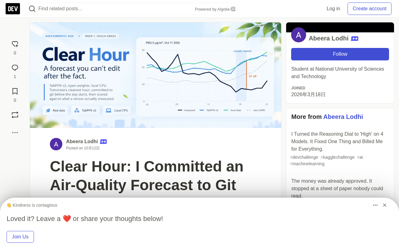
The open-source project, called Clear Hour, is built around Prior Labs' open-source tabular foundation model TabPFN v2, running entirely on a laptop CPU. And the author leads with her most embarrassing finding: on the very first day tested against real data, all three models — including TabPFN — ranked the 24-hour cleanliness window completely backwards.

A Real Problem Worth Solving

"Go outside for a walk" is good advice in most places — but in Islamabad, once the seasonal smog arrives in October, that advice deserves scrutiny. The author notes that local air quality apps only show "today's number" — a stale figure that compresses a 4× intraday swing into a single colored badge.

Clear Hour takes a different approach: it ranks tomorrow's full 24 hours by air cleanliness, identifies the best two-hour window for going out, and flags the worst periods to avoid.

The real discipline lies in temporal ordering. It's far too easy to run predictions on a day that "happened to go well" and write a glowing post afterward. So the author set an iron rule: a day's forecast must be committed to Git before that day begins, and the file may never be touched afterward. When the day ends, an independent script fetches real measurements and scores everything — no matter how ugly.

Honest Results: The Rankings Were Completely Reversed

On the day tested, the sensor's all-day average was 45.4 µg/m³. The actual cleanest two-hour window was 17:00–19:00 (20.9 µg/m³); the worst was midnight (79.2 µg/m³).

Here's how the three models performed:

Model	MAE	Bias	Spearman (24h)	Chosen Cleanest 2h	Actual Value
B0 Raw CAMS	21.9	−3.5	−0.512	05:00–07:00	73.7
M1 TabPFN v2	21.9	+14.6	−0.369	15:00–17:00	29.8
B2 CAMS+hourly bias	25.3	+18.8	−0.409	15:00–17:00	29.8

Every Spearman value is negative, meaning the models' rankings were the opposite of reality — the times they rated cleanest were actually dirtier. Raw CAMS made the most dangerous mistake of all: it recommended going out at 5 a.m., which happened to be the second-dirtiest two-hour window of the day. TabPFN and B2 at least selected windows below the daily average, but both missed the true window by two hours and badly underestimated how clean the evening air would become.

The author puts it plainly: "On the only day this project has been tested against reality, it ranked the hours backwards." But she also emphasizes this is not a final verdict on TabPFN — one day is one sample. Doing well tomorrow would prove just as little. The real evidence comes from the 30-day holdout evaluation that follows.

The Tech Stack: Fully Open, Fully Auditable

The entire pipeline is built from three free, open-source components:

• Air quality forecasts: CAMS global model via Open-Meteo, hourly PM2.5
• Meteorological forecasts: Open-Meteo boundary layer height, wind, humidity, temperature, precipitation — features that explain why CAMS is wrong
• Ground truth: Real sensors from OpenAQ v3, located 5.2 km from the CAMS grid point

CAMS is a serious atmospheric model, but at this specific location it is predictably wrong: it reads an average of 18.9 µg/m³ low relative to the reference monitor, and its error depends strongly on hour and season — from October through December, it can be off by 90 µg/m³ at the morning 9 a.m. peak. This structured, recurring error is exactly the kind of thing a tabular model can learn.

Three Models Shown Side by Side — Weak Baselines Not Quietly Dropped

Every forecast card shows all three models simultaneously: raw CAMS (control), CAMS plus per-hour bias correction (a deliberately one-line baseline), and TabPFN v2 running on a local CPU.

TabPFN is used with admirable restraint — no fine-tuning, no hyperparameter search, no hosted API. The key parameter is ignore_pretraining_limits=True: TabPFN v2 by default refuses training sets larger than roughly 1,000 rows, and pushing to 10,000 rows is exactly why a single fit takes 30–90 minutes instead of seconds. The first fit on the author's laptop took 3,351 seconds (56 minutes), after which the model is cached to disk (~6.3 GB for 10,000 rows) and can be reloaded in about 2 minutes.

CAMS (Copernicus Atmosphere Monitoring Service) is a global atmospheric composition forecasting system operated by ECMWF under the EU's Copernicus programme. It provides hourly global gridded data for PM2.5, PM10, ozone, nitrogen dioxide, and more at roughly 40 km spatial resolution, available free of charge. Due to its grid resolution, CAMS cannot capture intra-city concentration differences caused by local terrain, traffic, or coal heating. In regions like South Asia with sparse monitoring infrastructure, its systematic biases tend to be larger and exhibit clear diurnal patterns. These "predictable errors" are the entry point for post-processing correction models — the model doesn't need to understand atmospheric physics, just learn the statistical relationship between bias and hour, season, and meteorological conditions. Open-Meteo is an open-source weather API project that unifies outputs from multiple public models (CAMS, ICON, GFS, etc.) into a single interface, requiring no registration or API key — removing a key barrier for independent developers without institutional resources.

When "Pre-registration" Collides with a 56-Minute Fit

A one-hour fit obviously doesn't fit inside the ideal "commit before the day begins" window. Rather than fudge it, the author split October 11's forecast into two clearly labeled commits:

• Local time 06:10:46: B0 and B2 committed from freshly fetched data
• Local time 06:51:41: TabPFN committed based on the same in-memory feature matrix — no re-fetch

The card states plainly: hours before 06:51 had already happened and don't count toward TabPFN's pre-registration. The scoring script reports both full-day results and a separate "≥07:00" view that re-derives each model's recommended window using only hours that were still in the future. The author is clear: "An ugly two-phase commit with honest annotations beats a clean story that implies the 56-minute model finished at midnight."

The scoring script only reads frozen forecasts and only writes new files. At the CLI level, a --force mechanism prevents overwriting existing pre-registered files — the numbers cannot be quietly adjusted after the fact, by anyone, including the author herself.

Pre-registration comes from academic research practice: before collecting data or observing results, researchers publicly record and lock down their hypotheses, analysis methods, and evaluation metrics — preventing post-hoc methodological adjustments (known in statistics as "p-hacking" or "HARKing"). In machine learning, the analogous problem is researchers iterating on models or features after seeing test results, then presenting the final version as if it were a single clean run. Committing predictions to a public Git repository transplants this academic norm into engineering practice: Git commits carry cryptographically signed timestamps, and anyone can verify a file's exact contents at a specific moment via its commit hash, fundamentally preventing after-the-fact tampering. This is why the "no overwriting pre-registered files" CLI mechanism matters so much — it enforces the rule at the code level, rather than relying on the author's self-discipline.

Where TabPFN Actually Wins — and Where It Doesn't

30-Day Holdout Evaluation: A Test Month Used Only Once

The author uses strict chronological splitting, with a 30-day test month that all models can see exactly once — the code refuses a second test run.

Model	MAE	RMSE	Intraday ρ (median)	Top-2h Hit Rate
B0 Raw CAMS	16.1	20.7	0.564	30%
B2 CAMS+hourly bias	22.1	28.7	0.544	43%
B5 HistGBR	10.8	15.2	0.644	40%
M1 TabPFN v2	10.3	14.6	0.675	37%

TabPFN has the lowest error, and its MAE advantage over B2 is solid (95% CI: −17.0 to −6.9). But its ranking advantage over B2 is not statistically significant at this sample size, and an untuned HistGBR actually beat it on the validation month. The author puts it directly: "I'd rather print these three caveats than print only a bolded win."

How Much Data Does TabPFN Actually Need?

This is perhaps the most interesting finding. Using six-fold rolling-origin learning curves, the author concludes: TabPFN v2 needs roughly 1,000–2,500 hours of training data (about 6–15 weeks) before it matches, let alone slightly beats, a one-line hourly bias baseline on hourly ranking. Below that threshold it performs worse and is less stable (at N=100, ranking fluctuates ±0.34 across folds).

For a foundation model celebrated for its few-shot capabilities, "you need six weeks of data to beat one line of arithmetic" is a genuinely useful negative result — and exactly the kind of finding that hackathon blog posts typically bury.

Another surprise: a correction trained on one sensor and applied without any retraining to another sensor about 5 km from the CAMS grid point still works (TabPFN MAE 16.8 / ρ 0.661, far better than raw CAMS at 27.5 / 0.570). This cross-sensor transfer capability has major implications for scaling the project.

Spearman rank correlation (ρ) measures the monotonic agreement between two rankings, ranging from −1 to +1: +1 means perfect agreement, 0 means no relationship, −1 means perfectly reversed. For the air quality window recommendation task, what users care about isn't absolute concentration accuracy (what MAE/RMSE measure), but whether the model correctly judges "slot A is cleaner than slot B" — which is exactly what Spearman ρ captures. On the first real test day, all three models had negative ρ values (roughly −0.4 to −0.5), meaning their ranking judgments were worse than random guessing, and their "cleanest" recommendations were actually some of the dirtiest periods of the day. A rolling-origin learning curve is the standard method for evaluating the data-quantity/performance relationship in time series: by progressively moving the training start point forward, you get multiple evaluation results at different training sample sizes — letting you observe how performance improves with accumulating data without leaking future information into the past.

TabPFN v2 (Tabular Prior-Fitted Network v2) is a tabular data foundation model developed by Prior Labs. Its core idea is to pretrain a Transformer on massive synthetic tabular datasets, enabling Bayesian-style posterior predictions at inference time without gradient updates — essentially passing training data as context into the network, similar to in-context learning in large language models. This gives it stronger inductive biases than traditional tree models in low-data regimes, but at the cost of inference compute scaling quadratically with training set size (Transformer attention complexity) — which is why 10,000 rows causes a 56-minute fit time. HistGBR (HistGradientBoostingRegressor) is scikit-learn's histogram-based gradient boosting implementation, similar in spirit to LightGBM. It trains very fast on medium-sized tabular data and typically achieves competitive performance with minimal tuning, making it one of the most natural baselines for evaluating whether more complex models are actually worth the trouble.

Why "Open" Is a Hard Requirement Here

For this project, openness isn't an abstract value — it's the entire reason the project can exist.

There's simply no product to buy. Pakistan has no public hourly air quality forecast service. Islamabad's only reference-grade monitor — the US Embassy BAM — stopped publishing data, with no replacement. No commercial vendor will build an hourly-resolution smog model for Rawalpindi; the market size doesn't support it. If anyone is going to build this, it has to be someone who lives there, piecing it together from open-source components.

Every layer is open, and every layer carries weight: CAMS is publicly funded atmospheric modeling, Open-Meteo makes its output queryable without a corporate contract, OpenAQ aggregates sensor data under open licenses, and TabPFN v2 has open weights that run on CPU — that last point genuinely changes the economics.

The author does the math explicitly: if TabPFN were a closed, metered, hosted API, the 56-minute fit cost would land on every city, every sensor, every retraining run. The project would die from unit economics before helping anyone. Because the weights are open and inference is local, the marginal cost of calibrating a new sensor is just "CPU time on hardware someone already owns." Combined with the cross-sensor transfer result, this means someone in Lahore or Peshawar can clone the repo, point it at their own OpenAQ sensor, and get a working predictor — no API key, no quota, no permission from anyone required.

Openness is also what makes honesty enforceable. Pre-registered forecasts only mean something when strangers can verify them — they're Git commits with timestamps, public hashes, and feature matrix checksums. Anyone can confirm that the October 11 forecast existed at 06:10 that day and was never edited afterward. You can't audit the track record of a closed forecaster; you can only read its marketing copy.

Mistakes the Author Made

The article includes a refreshingly candid list of "here's what I got wrong" — more valuable than any success list:

• A bad compute budget estimator used quadratic extrapolation to misestimate large experiment runtimes, silently skipping the largest experiments — the real cost was only 12–22 minutes
• The author assumed TabPFN v2 weights were pure Apache-2.0. They're not — it's the Prior Labs License 1.1, which requires displaying "Built with PriorLabs-TabPFN" anywhere the weights or their outputs appear. She had to retroactively add attribution to the README, CLI, and demo page
• The real-time feature matrix behind the October 11 prediction was never written to disk or hashed, creating an audit gap that couldn't be handed to skeptics (every subsequent run now saves and hashes it)
• requirements.txt only installs cleanly on the author's machine — PyTorch CPU index configuration causes failures on a clean clone

"An open license is still a license," the author writes. "'Open' does not mean 'no obligations.'"

Honesty Is the Methodology

Clear Hour's technical highlights — running an open-source foundation model on a local CPU, correcting structured biases in a public atmospheric model, zero-retraining cross-sensor transfer — are all worth attention. But what's truly rare about this project is how it encodes verifiable honesty into the architecture itself: pre-registration, a one-shot test month, reporting failures, publishing confidence intervals, explicitly stating "this advantage is not significant."

As the author notes, the negative results in this article were published precisely because the architecture makes hiding them harder than publishing them. In a technical landscape saturated with cherry-picked results and post-hoc narratives, a project willing to publicly announce in the same article that it "ranked everything backwards" actually ends up building more credibility, not less.