PyTorch Image Classification in Practice: Complete Pipeline from Data Preprocessing to Model Training

Introduction

Image classification is one of the most classic tasks in computer vision and an essential milestone on the path to learning deep learning. Image classification refers to the task of having a computer automatically determine which predefined category an image belongs to. It is the cornerstone of Computer Vision because many more complex visual tasks (such as object detection, semantic segmentation, and instance segmentation) can be viewed as extensions of image classification. Since AlexNet won the ImageNet competition in 2012, Convolutional Neural Networks (CNNs) have become the standard approach for image classification, automatically learning hierarchical feature representations of images through convolutional layers—from low-level edges and textures to high-level object parts and semantic concepts—eliminating the tedious process of manually designing features in traditional methods.

This article will provide a detailed walkthrough of how to use PyTorch to complete the entire pipeline from data preprocessing, data augmentation, and model building to training and testing, based on a flower classification project.

More importantly, this pipeline serves as a universal template—whether you later work on image segmentation, object detection, or other visual tasks, the core approach to data preprocessing and training strategies remains the same, with the only difference being the network architecture in the middle.

Project Overview: 102-Class Flower Classification Task

Dataset Directory Structure

This project uses a flower dataset containing 102 categories (Flower Data), with a very intuitive directory structure:

• flower_data/train/: Training set, containing 102 subfolders numbered 1 to 102, each corresponding to a flower category
• flower_data/valid/: Validation set, same structure as the training set but with fewer samples per category

This dataset originates from the Oxford 102 Flower Dataset published by the Visual Geometry Group at the University of Oxford, created by Maria-Elena Nilsback and Andrew Zisserman in 2008, containing 102 common British flower species. The challenge of this dataset lies in the fact that different flower categories may look very similar (e.g., different varieties of daisies), while within the same category there can be significant intra-class variation due to different shooting angles, lighting conditions, and blooming stages. This makes it one of the classic benchmarks for Fine-Grained Visual Classification.

Data Volume Analysis and Strategies

A key issue is that the training set contains only about 6,000 images distributed across 102 categories, averaging fewer than 60 images per category. This data volume is relatively small.

The good news is that we can compensate for insufficient data through data augmentation strategies, while leveraging the transfer learning capabilities of pretrained models to achieve good results even on small datasets. The core assumption of Transfer Learning is that low-level visual features learned on large-scale datasets (such as ImageNet's 1.28 million images across 1,000 categories)—like edge detection, texture recognition, and color patterns—are universal and can be directly reused for new tasks. In practice, there are typically two strategies: one is to freeze most layers of the pretrained model and only train the final classification head (Feature Extraction); the other is to initialize the entire network with pretrained weights and then fine-tune all layers with a smaller learning rate (Fine-Tuning). For small datasets, transfer learning effectively prevents overfitting while significantly reducing training time.

Core Dependencies and Model Selection

Importing Key Modules

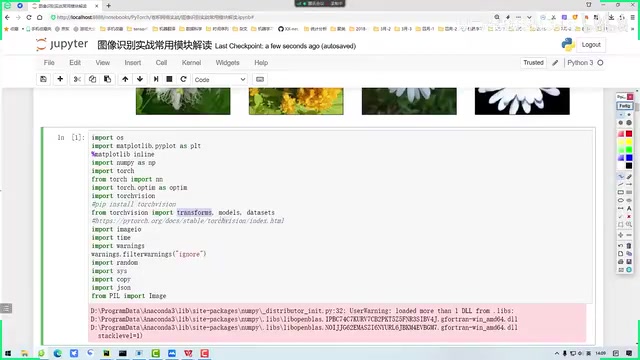
The project primarily depends on two core packages: torch and torchvision. Among them, torchvision provides three key modules:

1. transforms: For data preprocessing and data augmentation
2. models: Provides pretrained classic network models
3. datasets: Conveniently loads datasets organized by folder structure (where the ImageFolder class automatically maps folder names to category labels)

Why Choose ResNet as the Base Model

For model selection, this project directly uses ResNet from torchvision.models rather than building a network from scratch. The reason is simple: ResNet is one of the most widely used and classic models in computer vision, extensively validated in practice, with performance far exceeding most self-designed network architectures.

ResNet (Residual Network) was proposed by Kaiming He et al. from Microsoft Research in 2015, solving the degradation problem of deep networks by introducing residual connections (Skip Connection/Shortcut Connection). In traditional deep networks, as the number of layers increases, training error actually rises—this is not overfitting but rather optimization difficulty. The core idea of ResNet is: let the network learn the residual mapping F(x) = H(x) - x, rather than directly learning the target mapping H(x). By directly connecting the input x to the output via a skip connection, even if some layers learn zero mappings, network performance won't degrade. This design makes it possible to train networks with hundreds or even thousands of layers. ResNet won the ImageNet competition with a 3.57% top-5 error rate, surpassing human-level performance (approximately 5.1%) for the first time, and has spawned variants of different depths including ResNet-18, ResNet-34, ResNet-50, ResNet-101, and ResNet-152.

For practical projects, standing on the shoulders of giants is the wise approach.

Data Preprocessing: Building a Universal Pipeline

Path Configuration

First, you need to specify the data paths. The code uses the data_dir variable to point to the flower_data directory, then concatenates the training and validation set paths:

data_dir = 'flower_data'
train_dir = os.path.join(data_dir, 'train')
valid_dir = os.path.join(data_dir, 'valid')

If you want to migrate this to your own project, simply organize your data in the same folder structure and modify the paths.

transforms.Compose: Combining Preprocessing Operations in Sequence

The core of data preprocessing is transforms.Compose, which combines multiple preprocessing steps in sequence into a pipeline. The processing strategies for training and validation sets are different—the training set requires data augmentation, while the validation set does not.

transforms.Compose adopts the Pipeline pattern from functional programming, chaining multiple data transformation operations into a single callable object. Each transformation operation receives a PIL Image or Tensor as input and returns the processed result as input for the next operation. The advantages of this design include: modularity (each transformation is independently reusable), composability (freely combining different transformations), and lazy execution (transformations are only executed when data is actually loaded, not by preprocessing all data in advance). In PyTorch's DataLoader mechanism, transforms are executed dynamically at each sampling, meaning the same image undergoes different random augmentations in different epochs, effectively expanding the training data volume.

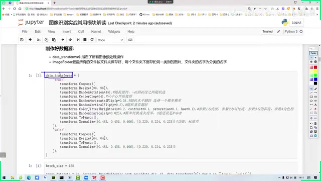
The code uses a dictionary structure to manage two preprocessing schemes:

data_transforms = {
    'train': transforms.Compose([...]),  # Training set: includes data augmentation
    'valid': transforms.Compose([...])   # Validation set: basic processing only
}

Resize: Unifying Input Dimensions

The first step in preprocessing is Resize. Original images have varying heights and widths, but convolutional neural networks require all input data to have the same dimensions, so all images must be resized to a fixed size.

This project uses a size of 96×96 (square), with several considerations behind this choice:

Size	Pros	Cons	Use Case
96×96	Fast computation, runs on CPU	Loses more detail	Quick experiments, CPU environment
224×224	Standard ResNet input, good results	Moderate computation	GPU environment
256×256+	Preserves more features	High computation, high VRAM demand	High-performance GPU

Resize Size Selection Guidelines:

• When training on CPU, choose 96 or 64, otherwise training time will be extremely long
• With a GPU environment, try 224 or 256 for significantly better results
• Larger sizes increase computation at every convolutional layer, and the cumulative difference across dozens of layers is enormous
• Square inputs are mainstream for classification tasks, and most classic networks are optimized for square inputs

It's worth noting that the computational cost of convolutional layers is proportional to the spatial dimensions of the input feature map. For a convolutional layer with kernel size k×k, input channels C_in, and output channels C_out, the floating-point operations (FLOPs) are approximately 2 × k² × C_in × C_out × H × W, where H×W is the spatial size of the output feature map. Therefore, increasing the input from 96×96 to 224×224 increases computation by approximately (224/96)² ≈ 5.4 times, and the cumulative effect across dozens of layers is very significant.

Data Augmentation: An Essential Strategy for Small Datasets

For a dataset with only about 6,000 images across 102 categories, data augmentation is almost mandatory. The theoretical foundation of data augmentation comes from regularization and invariance learning: from a regularization perspective, data augmentation constrains the model's hypothesis space by artificially increasing training sample diversity, reducing overfitting risk, with effects similar to L2 regularization or Dropout; from an invariance learning perspective, by applying various geometric and photometric transformations to images, the model is forced to learn feature representations that are invariant to these transformations. Research shows that proper data augmentation strategies can improve model accuracy by 5-15 percentage points, with particularly significant effects on small datasets.

The transforms module provides a rich set of augmentation methods, commonly used ones include:

• RandomResizedCrop: Random crop and resize, simulating different shooting distances. This operation first randomly selects a sub-region of the original image (with area ratio and aspect ratio randomized within specified ranges), then scales it to the target size, achieving both position augmentation and scale augmentation simultaneously
• RandomHorizontalFlip: Random horizontal flip, increasing sample diversity. Flipping is performed with a default probability of 50%, particularly effective for left-right symmetric objects like flowers
• RandomRotation: Random rotation, improving model robustness to angle variations
• ColorJitter: Color jittering (brightness, contrast, saturation), simulating different lighting conditions. This is especially important for outdoor flower photos, as natural lighting conditions vary greatly
• Normalize: Normalization (using ImageNet mean and standard deviation), accelerating model convergence

Regarding the Normalize operation, it converts image pixel values from the [0,1] range to a distribution centered around 0 with standard deviation near 1. The commonly used ImageNet normalization parameters in PyTorch are mean=[0.485, 0.456, 0.406], std=[0.229, 0.224, 0.225], which are the RGB channel means and standard deviations computed from ImageNet's 1.28 million images. Normalization places the input data distribution near the origin with consistent variance across dimensions, helping gradient descent optimizers work more efficiently. When using pretrained models, you must use the same normalization parameters as during pretraining, otherwise the shift in input distribution will cause pretrained features to fail.

It's important to note that data augmentation should only be applied to the training set. The validation set should only undergo basic operations like Resize and Normalize to ensure objective evaluation results. This is because the purpose of the validation set is to simulate model performance in real-world scenarios—if random augmentation is also applied to the validation set, evaluation results will lack reproducibility and comparability.

In recent years, automated methods have emerged in the data augmentation field, such as Google's AutoAugment (searching for optimal augmentation strategies through reinforcement learning) and RandAugment (randomly selecting augmentation operations with unified intensity control), which further reduce the cost of manual hyperparameter tuning.

Summary and Practical Recommendations

This article covered the first half of a PyTorch image classification project—data preparation and preprocessing. Key takeaways:

1. Universal template mindset: Data preprocessing and training strategies are highly transferable across classification/segmentation/detection tasks—learn one and apply to all
2. Leverage pretrained models: Classic models like ResNet have been thoroughly validated; using them directly is far superior to designing your own
3. Resize size trade-offs: Find the balance between computational resources and model performance
4. Data augmentation is an essential skill: Especially for small dataset scenarios, proper data augmentation can significantly improve model performance

For beginners, it's recommended to first run through the entire pipeline with a small size (96×96) to understand the purpose of each step, then gradually increase the size and try different augmentation strategies to optimize results. The code and dataset for this entire project can be run directly, making it an excellent hands-on project for getting started with deep learning.

Key Takeaways