PyTorch Tensors from Beginner to Practice: A Complete Guide to Core Concepts and Operations

Understanding tensors is the foundation of building neural networks with PyTorch. Many beginners rush to build models while overlooking the essence of tensors as data containers. This article, based on a complete PyTorch hands-on tutorial, systematically organizes the core concepts and high-frequency operations of tensors to help you lay a solid foundation before writing any network code.

What Exactly Is a Tensor? From Scalars to High-Dimensional Data Containers

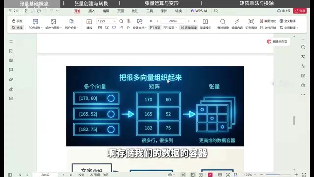
The tutorial opens by clarifying a key insight: in PyTorch, scalars, vectors, and matrices can all be uniformly called tensors. A vector is a one-dimensional tensor, a matrix is a two-dimensional tensor, and a tensor itself can be understood as a multi-dimensional data container with a shape. This definition seems simple, yet it determines the logic of all subsequent operations.

Understanding tensors requires grasping three basic concepts. Rank refers to how many axes a tensor has—the number of axes is the rank. Axis refers to the dimension along each direction, similar to the X, Y, and Z axes in a mathematical coordinate system. Shape describes the size along each dimension. A scalar has no shape because it is just a single number; a three-dimensional vector has shape 3; a matrix with three rows and four columns has shape (3, 4); and a tensor with shape (2, 3, 4) can be understood as two three-by-four matrices stacked together.

The tutorial repeatedly emphasizes one way of understanding: the essence of a matrix is putting many vectors together for convenient one-shot computation. A single vector represents one object—such as a person's height and weight, or a house's area, floor, and price. Multiple objects form a matrix. If you also need to represent people from different classes, you need to introduce the class as a new dimension, which naturally leads to a three-dimensional tensor.

Why Turn the Real World into Tensors

This is a particularly insightful passage in the tutorial. Text, images, vehicles, roads, pedestrians, and traffic lights in the real world cannot be "seen" by the model itself. The model runs on a computer, and computers only understand numbers. Therefore, the first step must be to turn these things into numbers so the model can compute, compare, judge, and learn.

In a vector, what we care about is not the numbers themselves but what the number at each position represents. The more complex the object, the more features are needed, and the higher the vector's dimensionality. Organizing vectors for multiple objects into a matrix, and then organizing multiple matrices into higher-dimensional tensors, all these containers ultimately serve the same purpose: making data easier to compute. In deep learning and large models, text and images are all converted into numbers and then into tensors, because tensors are the unified container through which models process numbers.

Creating Tensors and Device Management

The code for creating tensors is very intuitive. Defining a scalar only requires passing in a single number; defining a vector means passing in a list; defining a matrix means passing in a two-dimensional array; defining a three-dimensional tensor means passing in a nested list. The tutorial offers a handy trick for determining dimensionality: count the opening brackets on the left—one bracket is one dimension, two are two dimensions, three are three dimensions.

Tensor operations can specify a device, typically CPU or GPU. By default, tensors are computed on the CPU. To use the GPU, first check whether CUDA is installed on your computer, then move tensors to the corresponding device via .to(device), or explicitly migrate them using .cuda() or .cpu(). The tutorial demonstrator's computer only has a CPU, so data.cuda() throws an error—a reminder that device migration requires hardware support.

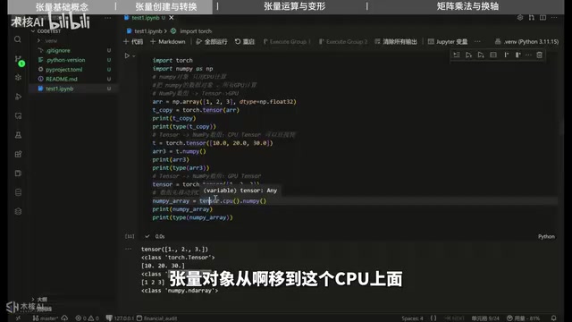
PyTorch also provides special tensor creation methods similar to NumPy: all-zero tensors, all-one tensors, randomly initialized tensors, identity matrices with ones on the diagonal, and direct calls to activation functions like Sigmoid, Tanh, and ReLU. The tutorial specifically reminds readers that these functions don't need to be memorized—just look them up in the PyTorch API when needed.

Converting between NumPy arrays and tensors is a common operation. NumPy's ndarray can only be computed on the CPU; to process such data on the GPU, you must first convert it to a tensor and then migrate it to the GPU. Conversely, a tensor on the CPU can be directly converted by calling .numpy(); a tensor on the GPU must first be moved with .cpu() before conversion.

CUDA (Compute Unified Device Architecture) is a parallel computing platform and programming model introduced by NVIDIA that allows developers to use the GPU's thousands of computing cores for general-purpose computing. In PyTorch, torch.cuda.is_available() is used to detect whether the current environment supports CUDA—that is, whether a compatible NVIDIA GPU exists and the driver and CUDA toolkit are correctly installed. If it returns False, any operation attempting to move tensors to the GPU (such as .cuda() or .to('cuda')) will throw a runtime error. Therefore, when writing cross-device code, it is common to first define device = torch.device('cuda' if torch.cuda.is_available() else 'cpu') and then uniformly use .to(device) to ensure the code runs in environments with or without a GPU.

Broadcasting: Computing with Different Shapes

Broadcasting is an unavoidable rule in tensor operations. Matrix addition usually requires matching shapes, but PyTorch allows automatic expansion under specific conditions. For example, when adding a matrix of shape (3, 1) to a matrix of shape (1, 2), the former copies its columns according to the latter's column count, and the latter copies its rows according to the former's row count; both are ultimately expanded to (3, 2) and then added element-wise. Similarly, when multiplying a vector of shape (1, 3) by a matrix of shape (2, 3), the vector is copied into two rows so the shapes align.

This mechanism was already introduced in the NumPy prerequisite course, and PyTorch follows the same design philosophy—understand it once and you can apply it everywhere.

Broadcasting is a mechanism introduced by NumPy that PyTorch fully inherits and uses for tensor operations. Its rules can be summarized as: compare dimensions one by one starting from the trailing (rightmost) dimension; if two dimensions are equal or one of them is 1, they are considered compatible. When compatible, the dimension of size 1 is expanded (logically copied) to match the size of the other dimension. For example, when adding shapes (3, 1) and (1, 2), the trailing dimensions 1 and 2 are compatible (1 expands to 2), and the next-trailing dimensions 3 and 1 are compatible (1 expands to 3), resulting in shape (3, 2). If a dimension is neither equal nor 1 (such as 3 and 4), an error is thrown. Broadcasting does not actually allocate memory to copy data; instead, it achieves virtual expansion through strides of 0, making it efficient and memory-saving.

reshape: Change Shape, Not Data

reshape is a high-frequency method in coding, and its core semantics are rearranging the same set of data into a new shape. It only changes the shape, not the data content or ordering.

There is an iron rule for using reshape: the total number of elements must stay the same. A vector of 12 elements can become three rows by four columns, or two rows by six columns, but cannot become five rows by three columns—because the latter requires 15 elements, and a mismatched total throws an error immediately. There are also rules for reordering: when a one-dimensional array [1, 2, 3, 4, 5, 6] becomes two rows by three columns, the first row is 1, 2, 3 and the second row is 4, 5, 6; when it becomes three rows by two columns, it is 1, 2 / 3, 4 / 5, 6.

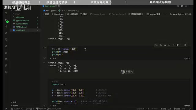
reshape also supports using -1 as a placeholder, meaning that dimension's size is automatically inferred by PyTorch based on the total number of elements. When passing (-1, 4), PyTorch divides 12 by 4 to get 3, equivalent to reshape(3, 4). The tutorial tested setting both dimensions to -1 on the spot, which resulted in an error—only one dimension can be inferred. This is worth noting for beginners.

Matrix Multiplication: Row-by-Column and Batch Operations

The dot product is an operation between two vectors, invoked with the dot method, and the result is a scalar. Cosine similarity is obtained by dividing the dot product by the product of the two vectors' magnitudes. Transposition swaps the rows and columns of a matrix; a three-by-two matrix becomes two-by-three after transposition.

Matrix multiplication has strict mathematical rules: if A has shape (M, N), then B must have shape (N, K), and the result C has shape (M, K). The tutorial demonstrates the "row-by-column" computation with a concrete example: the value at the first row and first column of the result matrix equals the sum of the products of corresponding elements from A's first row and B's first column; the first row and second column uses A's first row times B's second column, and so on. There is no "why" to this rule—it is a mathematical definition, and violating it throws an error.

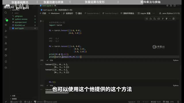
PyTorch offers two ways to write matrix multiplication: the @ operator and torch.matmul. The tutorial demonstrates that directly multiplying matrices with mismatched shapes throws an error, and that transposing one of the matrices makes it succeed.

There is also the bmm method, designed specifically for batch matrix multiplication, which requires the input to be a three-dimensional tensor. Passing two two-dimensional tensors directly to bmm throws an error. The tutorial recommends prioritizing the more general matmul for everyday matrix multiplication because it has better dimensional compatibility.

torch.bmm (Batch Matrix Multiplication) requires the input to be three-dimensional tensors of shapes (b, n, m) and (b, m, p), producing output of shape (b, n, p)—that is, performing two-dimensional matrix multiplication independently for each batch, with no data sharing between batches. torch.matmul (or the @ operator) is more general: for two-dimensional tensors, it performs standard matrix multiplication; for higher-dimensional tensors, it treats the last two dimensions as matrix dimensions and the preceding dimensions as batch dimensions, automatically applying broadcasting rules. For example, multiplying shapes (2, 3, 4) and (4, 5) yields shape (2, 3, 5). Therefore, when handling batch data or uncertain dimensions, matmul is the safer choice; bmm is suitable for explicit three-dimensional batch scenarios and offers slightly better performance.

Axis Swapping: Understanding Changes in Index Order

Axis swapping is slightly more complex than the previous operations. Swapping axes on a two-dimensional array is essentially transposition—rows and columns swap; a vector has only one axis, so no axis swapping applies. The concept of axes can be compared to a coordinate system: a matrix's rows are axis 0 and columns are axis 1; an axis essentially describes the order in which indices are accessed.

Take a concrete element as an example: a value is at the second row and second column, indexed as (1, 1). After swapping axes, the original rows become columns and columns become rows, and the same element now needs to be indexed as (1, 0)—the access order changes accordingly. This is what it means for axis swapping to change the index order.

PyTorch provides two axis-swapping methods: transpose and permute. transpose can only swap two dimensions, while permute can rearrange all dimensions in any order at once. For swapping axes on three- or four-dimensional tensors, permute is clearly more convenient. The tutorial admits that axis swapping on three- and higher-dimensional tensors is more troublesome to understand, but once you grasp the intuition of two-dimensional transposition, generalizing to higher dimensions is not difficult.

transpose(dim0, dim1) swaps the two specified dimensions and returns a new tensor view (without copying data), but after swapping, the tensor may no longer be contiguous in memory, in which case calling .view() throws an error and you must first call .contiguous(). permute(*dims) accepts a permutation of dimension order and rearranges all dimensions at once; for example, calling permute(2, 0, 1) on a tensor of shape (2, 3, 4) yields shape (4, 2, 3). Both return views, and modifying the view affects the original tensor. If you need an independent copy, use .clone(). The key to understanding axis swapping is this: it changes the order of dimensions, thereby changing how index tuples are interpreted, but the physical arrangement of elements in memory may remain unchanged (for transpose) or be reinterpreted in the new order (for permute).

Final Thoughts

This tutorial covers core operations including tensor concepts, creation, device management, broadcasting, reshape, matrix multiplication, and axis swapping—almost all of which are used daily in practice. For learners who want to build neural networks with PyTorch, solidifying these fundamentals is far more valuable than rushing to call model APIs. When you encounter an unfamiliar function, consulting the official API documentation is the most efficient path—there is no need to memorize everything by rote.