QGIS + Sentinel Radar-Optical Fusion: High-Precision Soil Moisture Mapping in Practice

Why Soil Moisture Monitoring Matters

Tracking surface soil moisture across large agricultural areas is essential for accurately modeling continental water cycles and ensuring global food security. Ground-based sensors deliver high-quality data but are geographically constrained, expensive to maintain, and impossible to scale. Satellite remote sensing, by contrast, provides the regional to planetary coverage required at a fraction of the cost.

Fields absorb and retain water, and when a region experiences a severe drought, crops can be destroyed before traditional monitoring systems ever detect the problem. Manually tracking moisture field by field across the globe is physically impossible. The only solution at that scale is continuous observation from space. This article breaks down a complete QGIS workflow for combining Sentinel radar and optical data to generate a color-coded soil moisture map at 10-meter resolution.

Why Radar Can Measure Moisture — and Why Vegetation Gets in the Way

Researchers rely on Synthetic Aperture Radar (SAR) — particularly the C-band instruments aboard ESA's Sentinel satellites — to collect data. The underlying physics: moisture dramatically changes the dielectric constant of soil. The more water present, the greater the soil's ability to store and reflect electromagnetic energy. This higher dielectric constant directly amplifies the intensity of radar backscatter. When a radar pulse strikes bare ground, the return signal is clean and directly correlated with soil water content.

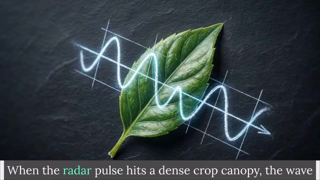
The problem is that most agricultural land is covered by a crop canopy for much of the year. When a radar pulse hits a dense canopy, the waves scatter in chaotic directions off leaves and stems, leaving only a faint signal to reach the ground. Two interference effects are at play: signal attenuation, where water in plant tissue absorbs some radar energy, and volume scattering, where radar waves bounce erratically through the plant's geometric structure. The result is that what the satellite receives is no longer a pure soil moisture signal but a mixture of ground data and vegetation noise. Applying a bare-soil algorithm directly will inevitably produce distorted results.

SAR is an active microwave sensor that images the surface by emitting microwave pulses and recording the echoes. Because it generates its own illumination, it can operate at night and penetrate cloud cover — a core advantage over optical satellites. The C-band wavelength of approximately 5.6 cm sits in the middle of the microwave spectrum, allowing partial penetration of vegetation canopies while remaining highly sensitive to soil moisture changes. Sentinel-1 operates in dual-polarization mode, acquiring both VV (vertical transmit, vertical receive) and VH (vertical transmit, horizontal receive) data simultaneously. VV polarization is more sensitive to surface scattering from the soil, while VH is more responsive to vegetation volume scattering. Together they provide complementary information that helps models distinguish the relative contributions of ground and canopy signals.

How the Water Cloud Model Works with Optical Data

The standard solution to the canopy problem is the semi-empirical Water Cloud Model (WCM), developed by Attema and Ulaby. Rather than modeling individual leaves, WCM treats the entire crop canopy as a uniform cloud of water droplets suspended above the ground. The model defines total radar backscatter as the sum of several components: a direct reflection contribution from the vegetation itself, and a soil contribution modified by a two-way attenuation factor — the soil signal is attenuated twice because the radar pulse must pass down through the canopy and back up again.

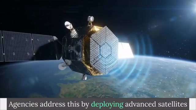
WCM depends on two unknown vegetation physical parameters (such as biomass and leaf area index) that cannot be solved mathematically from SAR data alone. The key is to bring in Sentinel-2 optical imagery: by computing the Normalized Difference Vegetation Index (NDVI) from red and near-infrared bands, you get a pixel-by-pixel canopy density map for the entire area. These NDVI values fill in the missing vegetation parameters in WCM, enabling the model to separate and subtract the canopy contribution from the total signal. The remaining soil contribution is then modeled using the Integral Equation Model (IEM) in combination with surface roughness.

NDVI is calculated as (NIR band − Red band) / (NIR band + Red band), with values ranging from −1 to 1. Healthy, dense vegetation — which strongly absorbs red light for photosynthesis while intensely reflecting near-infrared — typically yields NDVI values between 0.6 and 0.9. Bare soil or sparse vegetation falls around 0.1 to 0.3, while water bodies produce negative values. NDVI works as a proxy for WCM vegetation parameters because it correlates strongly with leaf area index (LAI) and vegetation water content — the two physical quantities that most determine how much the canopy attenuates the radar signal. Sentinel-2 provides 10-meter resolution red and near-infrared bands, closely matching the spatial resolution of Sentinel-1 SAR data and enabling pixel-by-pixel fusion.

From Physical Models to a Neural Network Data Pipeline

Solving these complex equations in real time for every pixel is computationally infeasible at scale. Instead, researchers use WCM and IEM to generate large synthetic training datasets covering soil moisture combinations from 2% to 40%, along with varying surface roughness and NDVI levels, with Gaussian noise injected to simulate real-world satellite imperfections.

This synthetic dataset is used to train an artificial neural network. The trained network takes four inputs — radar backscatter in VV and VH polarizations, local incidence angle, and optical NDVI — runs them through hidden layers, and outputs volumetric soil moisture percentage for each spatial unit. This pipeline effectively bridges the gap between theoretical physics and large-scale data engineering: the physical models provide the principles, and AI transforms them into a fast, scalable global data pipeline.

Training neural networks on synthetic data is a common strategy in remote sensing for addressing the "labeled data scarcity" problem. Ground-truth soil moisture sensors are limited in number and unevenly distributed, so training directly on observational data introduces severe geographic bias. Physical models like WCM + IEM can generate theoretical backscatter values under any parameter combination based on known electromagnetic scattering principles, constructing a training set that spans a wide parameter space. Gaussian noise is injected to simulate the inherent speckle noise in real SAR imagery — a granular texture caused by random interference of coherent microwave signals and an intrinsic characteristic of SAR images. Models trained on overly "clean" data tend to be brittle during real-world inference.

Breaking Down the QGIS Workflow

Following this workflow requires a configured QGIS environment with the Orfeo Toolbox, plus a Python environment containing libraries such as GDAL, Keras, and NumPy. The core steps are as follows:

Preprocessing and Masking

The study site landscape is highly fragmented, with target farmland interspersed with urban areas and water bodies. Start by applying a mask from a land cover map using the raster calculator to remove all urban and water regions. For radar data, it is recommended to use pre-calibrated orthorectified imagery from Google Earth Engine, bypassing raw Copernicus images and avoiding complex manual radiometric calibration.

Segmentation and Geometry Refinement

Apply mean-shift segmentation to the NDVI optical imagery, dividing the agricultural landscape into homogeneous spatial units based on an NDVI variation range of ±0.1. Creating uniform units is critical — mixing different vegetation types in a single calculation contaminates the radar signal characteristics. Then apply a smoothing geometry tool to round polygon vertices, followed by a fixed-distance negative buffer of 10 meters to keep calculations away from edge noise from roads, hedgerows, and similar features.

Statistical Extraction and Filtering

Use zonal statistics to count the number of pixels within each feature, and delete polygons with fewer than 20 radar pixels to eliminate random fluctuations from speckle noise. For retained features, extract VV and VH polarization values, local incidence angle, and NDVI, then export as a CSV file. Strict geometric filtering ensures that what enters the model is a clean soil signal, free from boundary mixing or random noise.

Computation and Mapping

Pass the CSV to Python and run the Apply Algo script (enter the filename in the Zonal Stat variable, then press F5 to launch the algorithm). The script automatically outputs the volumetric soil moisture percentage for each spatial unit. Return to QGIS to perform a table join, matching results to the segmented polygons, then apply a color gradient classification to the moisture data at 5% volumetric intervals.

A Real-World Example: From Drought to Saturation

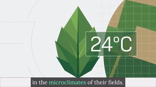
Take a 15×15 km agricultural site near Montpellier, France. On January 19th, after 19 consecutive days without precipitation, the site was dry and the map showed widespread moisture levels of 5% to 15%. One week later, on January 26th, 23 mm of heavy rain over the preceding four days dramatically transformed the landscape. The model detected saturation states of 30% to 40%, successfully penetrating the wet canopy to complete the observation.

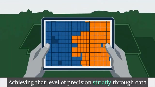
The distinct color variation between parcels demonstrates the success of the segmentation in achieving within-field-scale moisture monitoring. The advantage of these 10-meter readings over the kilometer-scale blind spots of earlier MODIS thermal sensors is immediately apparent. When validated against ground-based physical sensors, the correlation data fusion approach keeps errors within tight bounds.

Edge Cases and Application Value

This approach is not universal. Highly fragmented landscapes or severely mixed agricultural areas can still evade the algorithm — for example, if a farmer irrigates a very small plot heavily but its thermal footprint is too small to shift the average value of the large pixel covering it, the decomposition chain will miss the event.

That said, mastering this multi-platform workflow enables the conversion of raw satellite data into actionable intelligence that directly supports precision irrigation strategies and water cycle research. For agricultural planners, this means identifying under-irrigated parcels early enough to prevent crop failure before losses occur. The critical breakthrough does not always come from newly launched satellites — it is often hidden in the mathematical relationships within data streams we are already collecting.

The Mixed Pixel Problem is pervasive in remote sensing: when a single pixel contains multiple land cover types, the extracted statistics represent a weighted average of all the signals and cannot accurately reflect the true state of any single class. Ten-meter resolution is already among the highest available for open commercial satellite data, but for smallholder farmers — who dominate agricultural areas globally with plots of 0.1 to 1 hectare — a single pixel can still straddle two fields with entirely different farming practices. Future higher-resolution satellites (such as commercial SAR constellations) or miniature SAR sensors mounted on drones may push this limitation to finer scales, but the associated data volumes and processing complexity will increase proportionally.