Sample-Splitting Choices in TMLE and AIPW: The Impact of Cross-Fitting and Repeated Splitting

Sample-splitting choices in TMLE and AIPW systematically affect interval coverage and require careful design.
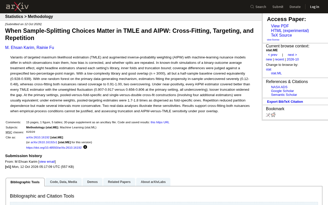
An arXiv simulation study systematically assessed how sample-splitting design in TMLE and AIPW (cross-fitting, targeting, repetition) affects interval coverage. With random forests for the main data-generating mechanism and in-sample propensity fitting, coverage fell to 0.12–0.48; cross-fitting both nuisances restored it to 0.91–1.00. Under near-positivity, all AIPW coverage rates (0.907–0.917) beat TMLE with unweighted fluctuation (0.656–0.806). Under extreme weights, pooled targeting was 1.7–1.8 times more dispersed than fold-specific targeting. Repeated splitting reduces reliance on a single split but makes intervals more conservative. The study recommends cross-fitting both nuisances when empirical-process conditions cannot be justified, and assessing truncation and reporting both AIPW and TMLE results when overlap is poor.
In the practice of causal inference, TMLE (Targeted Maximum Likelihood Estimation) and AIPW (Augmented Inverse-Probability Weighting) are often treated as "plug-and-play" robust methods—as long as you connect a machine learning model, you get double robustness. But a simulation study published on arXiv offers a more nuanced warning: the sample-splitting scheme itself is a design dimension that cannot be ignored. Whether cross-fitting is used, how the targeting step is performed, and whether repetition is applied all systematically change the interval coverage of the estimators.
Study Design: A Controlled Experiment with Known Ground Truth
This study uses a simulation framework with known ground truth to evaluate the average treatment effect (ATE) for binary outcomes. Eight "headline" estimators share the same nuisance model library, number of internal folds, and truncation bound under the same setup, so that differences can be attributed to the sample-splitting strategy itself. Coverage is judged against two pre-specified percentage-point margins: only deviations beyond this range count as a "substantive difference," avoiding the mistake of treating Monte Carlo noise as a conclusion.
The simulations are divided into three levels of difficulty. The first level is a low-complexity model library with good overlap (n=3000); here, apart from the half-sample baseline, all estimators have coverage between 0.928 and 0.939, making them equivalent to one another. The second level switches to random forests for the main data-generating mechanism, and the situation deteriorates sharply: estimators that fit the propensity score in-sample see coverage drop to 0.12–0.48, severe undercoverage; once both nuisances are cross-fitted, coverage recovers to 0.91–1.00, with two estimators even showing overcoverage. The third level is a near-positivity setting, where every AIPW estimator has better coverage than every TMLE estimator using an unweighted fluctuation, with a gap of 0.907–0.917 versus 0.656–0.806 in the main setting, and all TMLE estimators show undercoverage; relaxing truncation widens the gap further.
Double robustness is the shared selling point of AIPW and TMLE: the estimator is composed of an outcome regression model and a propensity score model, and as long as one of them is correctly specified, the ATE estimate is consistent. This property mathematically depends on the convergence rates of the two nuisance functions and empirical-process conditions, so its practical performance depends heavily on how the machine learning models are fitted. Nuisance functions are auxiliary functions that we do not directly care about but must estimate in order to estimate the target parameter—here, the outcome regression function and the propensity score function; TMLE removes the bias caused by nuisance estimation error by applying a "targeting update step" to the initial estimate.
Cross-Fitting: Not Optional, but a Default Premise
The most practically valuable finding from the above results is this: when empirical-process conditions cannot be rigorously justified, both nuisances should be cross-fitted simultaneously. The reason is not abstract—fitting the propensity score in-sample creates dependence among individual contributions, so variance estimates derived under the i.i.d. assumption underestimate true uncertainty. High-variance, strongly data-adaptive models like random forests amplify this dependence, so it is no surprise that coverage collapses to 0.12–0.48.
Cross-fitting splits the sample into folds, trains on the other folds, and evaluates on the held-out fold, restoring approximate independence among contributions. The study shows that this operation not only repairs coverage but, in some settings, slightly over-covers, which is a conservative but safe direction. For those doing real data analysis, this means that when overlap is moderate and model complexity is high, one should not skip cross-fitting just to save computation.
Empirical-process conditions are the technical prerequisites that ensure cross-fitted estimators are asymptotically normal and that variance estimates are valid; intuitively, they require that the complexity of the nuisance estimates not be too high, otherwise the variance formula based on the i.i.d. assumption fails. Positivity, also called overlap, means that every covariate value has a nonzero probability of being observed in each treatment group; when the propensity score approaches 0 or 1, weights become extremely inflated and variance rises sharply. A truncation bound is simply artificially restricting the propensity score to an interval such as [0.01, 0.99], trading a small amount of bias for variance stabilization; this choice itself also affects coverage, so the study recommends sensitivity analysis when overlap is poor.
Targeting Approach: The Trade-off Between Pooled and Fold-Specific
The study also compares pooled versus fold-specific targeting, and single versus double cross-fitting constructions, involving an additional four estimators. In the main setting, these variants are usually equivalent; but under extreme weights, the dispersion of estimates from pooled targeting is 1.7–1.8 times that of fold-specific targeting. The reason is that pooled targeting pools residuals from all folds together for updating, so individual high-weight observations can disproportionately influence the overall update; fold-specific targeting confines this influence locally.
This suggests a practical rule: when the tail of the weight distribution is very heavy, fold-specific targeting is more stable; when weights are moderate, pooled targeting has smaller variance because it uses all the data, and the two are not significantly different.
The targeting step is the key difference between TMLE and AIPW: AIPW directly applies a one-step correction to the initial estimate, whereas TMLE updates the initial outcome regression by fitting a fluctuation model with propensity weights as a covariate, so that the updated estimate satisfies the efficient influence function equation. The fluctuation model typically uses logistic regression for binary outcomes and linear regression for continuous outcomes, with its only covariate constructed from the propensity score. Pooled targeting concatenates residuals from all cross-fitting folds and updates once, while fold-specific targeting updates each fold separately. The influence function determines the asymptotic variance of the estimator; the efficient influence function after cross-fitting depends on averaging across folds, which is also why the number of folds and the splitting scheme affect interval width.
Repeated Splitting: Robust but Conservative
Repeated sample splitting averages results over multiple random splits, reducing dependence on any single split—this is its core value, especially when sample size is limited and the influence of split randomness is large. But the cost is that averaging over multiple intervals makes the overall result more conservative, and the study observes widening intervals for several estimators. In other words, repeated splitting buys stability at the expense of some efficiency. Whether it is worth it depends on the analytical goal: if the focus is reliability of interval coverage, repeated splitting pays off; if the focus is interval width and testing power, then computational cost and conservativeness must be weighed.
Implications for Practice
Two real-data analyses corroborate the above sensitivities, showing that these patterns are not simulation artifacts. Overall, the study gives two clear recommendations: first, when empirical-process conditions cannot be justified, use cross-fitting for both nuisances; second, when overlap is poor, proactively assess the choice of truncation bound and report results for both AIPW and TMLE, rather than selecting only one.
For researchers using machine learning for causal inference, the significance of this work is that it elevates "sample splitting" from an implementation detail to a design choice that needs to be reported and subjected to sensitivity analysis. Simply stating that TMLE or AIPW was used is far from sufficient—how you split, at which step you cross-fit, and where you set the truncation all directly determine whether the conclusions are credible.
When reporting causal inference results, sensitivity analysis should cover at least three dimensions: the number of folds (e.g., 2, 5, 10), the targeting approach (pooled or fold-specific), and the truncation bound (e.g., 0.01, 0.025, 0.05). One can use repeated cross-fitting to report empirical performance of interval averages and coverage, thereby explicitly incorporating sample-splitting uncertainty into inference. For settings with high demands on credibility, such as medicine and economics, it is advisable to report intervals for both AIPW and TMLE and explain the sources of possible divergence under extreme weights, so that reviewers and readers can judge the robustness of the conclusions.
One-line Summary
Sample-splitting choices in TMLE and AIPW systematically affect interval coverage and require careful design.
Paragraph Summary
An arXiv simulation study systematically evaluated how sample-splitting design in TMLE and AIPW (cross-fitting, targeting approach, repetition) affects interval coverage. Results show that when random forests are used for the main data-generating mechanism and the propensity score is fitted in-sample, coverage drops from normal levels to 0.12–0.48; cross-fitting both nuisances restores it to 0.91–1.00. Under near-positivity, all AIPW coverage rates (0.907–0.917) outperform TMLE with unweighted fluctuation (0.656–0.806). Under extreme weights, the dispersion of estimates from pooled targeting is 1.7–1.8 times that of fold-specific targeting. Repeated splitting reduces dependence on a single split but makes intervals more conservative. The study recommends cross-fitting both nuisances when empirical-process conditions cannot be justified, and assessing the truncation bound and reporting both AIPW and TMLE results when overlap is poor.
Related articles

@ai-sdk/vue 3.0.306 Patch Release Syncs with [email protected] Update
@ai-sdk/vue 3.0.306 released, synced with [email protected]. A routine patch release for the Vercel AI SDK ecosystem with no public API changes; the Vue adapter layer stays version-aligned with the core package.

Gemini 4 Argon API Launches: The Era of Million-Token Output Begins
Google launches Gemini 4 Argon with sparse MoE architecture, up to 1M output tokens, and a 68.90% Vals Index score, available across API, AI Studio, and the Gemini app.

DukaanAI: Turning Product Photos into Inventory Lists with Open-Source AI
DukaanAI is an AI inventory tool for small retailers that turns product photos into inventory entries using the open-source Gemma 3 model, with local inference, editable fields, and CSV export.