SVM Training Taking 10 Minutes? A Deep Dive into Grid Search Performance Pitfalls for Beginners

Why your SVM grid search is slow — and how to fix the combinatorial explosion causing it.
A beginner's SVM classifier took 10+ minutes on just 8,000 samples. The culprit wasn't SVM itself, but a 144-combination parameter grid multiplied by 5-fold cross-validation and per-class loops, producing 3,600 training runs. Add probability=True overhead and redundant kernel-parameter combos, and slowness is inevitable. The fix: trim the grid, use native multi-class support, and enable parallel training.
The Problem: Why Is a Small Dataset Running So Slowly?
A machine learning beginner posted for help on Reddit: they had built an SVM classifier with pandas, and after PCA dimensionality reduction and standardization, the dataset had only 2–3 features (10 at most) and at most 8,000 samples — yet training took at least 10 minutes. Even more puzzling was seeing others run through datasets with 400,000 rows × 1,000 features in just a few minutes.
In an attempt to "optimize," they reduced the sample size to around 200 and devised a complex sampling scheme — taking the max and min of each feature per class, then randomly padding to reach 200 samples. The result? The program didn't get faster — it got even slower. This "more optimization, more slowness" phenomenon reveals a classic blind spot in how beginners approach ML engineering.
Even running on a high-end gaming PC, they felt only a few hundred operations were completing per minute — far from the tens of thousands per second they expected. In reality, there are several precisely identifiable performance issues hiding beneath the surface.
Root Cause Analysis: It's Not SVM That's Slow — It's the Combinatorial Explosion in Grid Search
The Multiplicative Trap in Parameter Grids
The real culprit slowing everything down is hiding in the param_grid:
param_grid = {
    'C': [0.1, 1, 10],            # 3 values
    'gamma': [1, 0.1, 0.01, 0.001],  # 4 values
    'kernel': ['linear', 'poly', 'rbf'],  # 3 values
    'degree': [1, 2, 3, 4]        # 4 values
}
Each parameter may seem to have only a few values, but GridSearchCV iterates over every combination: 3×4×3×4 = 144 parameter combinations.
GridSearchCV is sklearn's core tool for hyperparameter search — it combines exhaustive enumeration of the parameter grid with k-fold cross-validation. The basic idea of cross-validation is to split the dataset into k equal parts, train on k-1 parts and validate on 1, then repeat k times and average the scores as the evaluation result for that parameter combination. While this improves reliability of model evaluation, it directly multiplies the number of training runs by k — and when the hyperparameter space is large, this combinatorial explosion catches many beginners completely off guard.
With cv=5 (5-fold cross-validation), each configuration requires training 144×5 = 720 models.
For a multi-class problem (say, 5 classes) using one-vs-all with a separate grid search per class, total training runs spike to 720×5 = 3,600. That's the core reason for the slowness — not that any single SVM training is slow, but that it's being repeated an enormous number of times.
The Hidden Cost of probability=True
SVC(probability=True) may look harmless in the code, but it comes at a steep price. SVM is fundamentally a discriminative model — its output is the distance from a sample to the decision hyperplane (the decision function value), not a probability. To convert this into probability output, sklearn uses Platt Scaling, a method proposed by John Platt in 1999: after SVM training is complete, it fits an additional Sigmoid function to map decision values to the [0, 1] range. This Sigmoid fitting itself requires internal cross-validation, which significantly increases the time cost of each fit call — and in a grid search scenario, this cost is multiplied across every combination. If you don't actually need probability outputs, simply removing this parameter will yield a noticeable speedup.
Redundant Parameter Combinations
Looking more closely at the parameter grid reveals logical waste: degree only applies to the poly kernel, yet grid search will iterate over all 4 degree values even for linear and rbf kernels, generating a large number of meaningless repeated training runs. Similarly, gamma is irrelevant for the linear kernel. These redundant combinations waste several times the compute budget unnecessarily.
The Sampling Logic: Why "Optimization" Made Things Slower
The developer's sampling code is another classic cautionary example. The intent was to "represent" the data distribution by taking the min and max of each feature plus random samples — but this approach has several obvious problems:
First, excessive print statements hurt performance. The code is full of debug-purpose print calls, frequently printing DataFrame contents inside loops. The I/O overhead in interactive environments like Jupyter is considerable.
Second, pandas idxmax/idxmin and repeated indexing operations are inefficient. Repeatedly calling data.iloc and pd.concat to concatenate DataFrames inside loops triggers a large number of unnecessary data copies.
Third, the sampling strategy destroys data representativeness. Forcing extreme-value samples into the training set introduces outliers, forcing SVM to construct more complex decision boundaries. High-degree poly kernels converge much more slowly on such data. This explains why the "carefully designed" sampling actually made the program slower — the hardest-to-classify boundary samples were deliberately packed in.
The right approach is to use StratifiedShuffleSplit or sklearn's built-in stratified sampling tools. Stratified Sampling is a foundational statistical method for preserving sample representativeness: samples are drawn in proportion to each class's share of the total population, ensuring the subset's class distribution matches the original dataset. sklearn's StratifiedShuffleSplit adds random shuffling and multiple resampling on top of this, making it especially suited for class-imbalanced scenarios. Compared to manually picking extreme-value points, stratified sampling preserves the statistical properties of the data, avoids artificially introducing outlier bias, and doesn't expose SVM to a deliberately constructed set of difficult training samples.
Practical Optimization Strategies
Trim the Parameter Grid and Eliminate Invalid Combinations
The most direct speedup is to reduce the parameter grid. You can use a list of dictionaries to specify valid parameters separately for each kernel:
param_grid = [
    {'kernel': ['linear'], 'C': [0.1, 1, 10]},
    {'kernel': ['rbf'], 'C': [1, 10], 'gamma': [0.1, 0.01]},
]
This completely eliminates the useless iteration over degree for non-poly kernels, cutting parameter combinations from 144 down to fewer than 10. The speedup is immediate and dramatic.
Use Native Multi-Class Support Instead of Hand-Written One-vs-All
sklearn's SVC already supports multi-class classification natively (using one-vs-one by default). There's absolutely no need to manually loop through each class and run a separate grid search. Just let GridSearchCV run once directly on the multi-class SVC — training runs drop by several times.
Enable Parallel Training with n_jobs
Adding n_jobs=-1 to GridSearchCV lets it take full advantage of a high-end PC's multi-core CPU to train different parameter combinations in parallel. This is especially effective for CPU-intensive grid searches.
Enable Probability Estimation Only When Needed
Only set probability=True when you genuinely need to call predict_proba. In all other cases, leave it at the default (disabled) to reduce the extra Platt Scaling overhead on every training run.
A Shift in Perspective: Why Does Someone Else's Larger Dataset Run Faster?
The developer's biggest source of confusion — how someone else can finish 4 million samples in a few minutes while 8,000 samples takes 10 minutes — actually has a clear answer: runtime is determined by the number of training runs multiplied by the complexity of each run, not by dataset size alone.
The other person was probably training just one or two models with fixed parameters, or using LinearSVC. Understanding the difference requires knowing SVM's time complexity: standard SVM (using optimization algorithms like SMO) has a training time complexity between O(n²) and O(n³) — going from 1,000 to 10,000 samples could theoretically increase training time by 100 to 1,000 times. LinearSVC, on the other hand, uses coordinate descent or dual coordinate ascent, with a time complexity closer to O(n), and runs far faster than kernel-based SVC in linearly separable or approximately linearly separable settings — it's a highly efficient specialized implementation for linear kernel scenarios. Additionally, the poly kernel requires computing high-degree polynomial mappings, making each kernel function evaluation far more expensive than rbf or linear, and when stacked across 3,600 repetitions, painfully slow performance is no surprise.
You might not have noticed, but SVM's training complexity does fall between O(n²) and O(n³) — yet for a few thousand samples, a single training run should be milliseconds. The slowness was never the SVM algorithm itself; it was layer upon layer of waste in engineering practice.
For machine learning beginners, this case offers a lesson far more valuable than its technical details: profile before you optimize — don't act on instinct. Use %timeit or simple timers to measure elapsed time section by section. More often than not, the actual bottleneck is the complete opposite of what your intuition suggested.
Key Takeaways
Related articles

Xi Jinping Proposes Open Source AI Cooperation Zone Among BRICS Nations
Xi Jinping proposed an open source AI cooperation zone at the BRICS summit. Analyzing the strategic intent, open source rationale, and global AI governance implications.
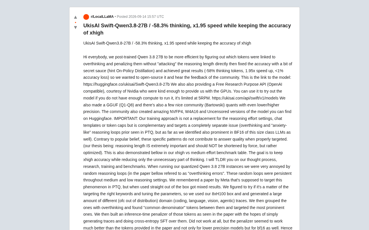
Swift-Qwen3.8-27B: 58% Fewer Thinking Tokens, Nearly 2x Faster Inference
UkisAI open-sources Swift-Qwen3.8-27B, cutting thinking tokens by 58% and boosting inference speed 1.95x via overthinking token penalties and on-policy distillation — with under 1% accuracy loss.

Netflix Partners with Sega: Crazy Taxi Movie and New Sonic Animated Series on the Way
Netflix announces three Sega game adaptations: a Crazy Taxi movie, a new Sonic animated series with edge, and a live-action film based on RGG Studio's Stranger Than Heaven.