Training Machine Learning Models from Scratch: A Complete Beginner's Guide

A beginner's complete guide to training your first ML model from scratch, from data prep to evaluation.
This guide systematically covers the full workflow of training a machine learning model from scratch: defining the problem type, preparing and preprocessing data, selecting algorithms, understanding the bias-variance tradeoff, tuning hyperparameters, and choosing evaluation metrics. It includes practical tool recommendations like scikit-learn and XGBoost to help programming beginners launch their first ML project.
Why Training ML Models Feels Daunting to Beginners
Across tech communities, you'll frequently come across posts like "Help me train a machine learning model." The question looks simple, but behind it lies a vast body of knowledge. For beginners, training an ML model means simultaneously tackling data processing, algorithm selection, hyperparameter tuning, model evaluation, and more—if any single link fails, the final result can suffer significantly.
This article systematically walks through the complete process of training a machine learning model from scratch, helping newcomers build a clear mental framework and avoid common pitfalls.
The Core Workflow of Training ML Models
Training an ML model is by no means as simple as "dump in the data and click run." A complete modeling pipeline typically involves several key stages, and understanding the logical relationships between them is the first step to getting started.
Step 1: Define the Problem Type
Before diving in, you first need to be clear about what type of problem you're solving:
- Classification: Predicting discrete labels, e.g., determining whether an email is spam
- Regression: Predicting continuous values, e.g., house price prediction
- Clustering: Grouping data in an unsupervised manner
- Recommendation/Ranking: e.g., a product recommendation system
The problem type directly determines your subsequent algorithm choices and evaluation metrics. Much of a beginner's confusion stems precisely from not having thought through "what exactly do I want the model to output."
It's worth noting that the taxonomy of machine learning problems is far richer than the four categories above. Supervised Learning relies on labeled data and encompasses classification and regression; Unsupervised Learning discovers structure in unlabeled data, including clustering, dimensionality reduction, and density estimation; Semi-supervised Learning leverages a small amount of labeled data alongside a large volume of unlabeled data for joint training, which is especially useful in domains where labeling is extremely costly, such as medical imaging. In addition, Reinforcement Learning learns policies through an agent interacting with an environment to maximize cumulative rewards, forming a cornerstone of recommendation systems and autonomous driving. Clarifying which learning paradigm a problem belongs to is a prerequisite for deciding your data labeling strategy, algorithm family, and evaluation scheme.
💡 Going Deeper: The Boundaries of the Four Learning Paradigms Are Blurring
With the rise of large-scale pretrained models, the boundaries between these paradigms are being redefined. Self-supervised Learning is one of the most influential new paradigms in recent years—it automatically constructs supervisory signals from the data itself (such as predicting masked words or predicting the rotation angle of an image), enabling the learning of high-quality representations without manual labeling. Groundbreaking models like GPT, BERT, and CLIP are all built on this idea. Understanding this evolution helps beginners quickly pinpoint the most suitable technical approach in real projects based on three dimensions: how much labeled data is available, how costly labeling is, and how large the dataset is.
Step 2: Data Preparation and Preprocessing
There's a long-standing saying in the industry: "Data sets the upper bound of model performance; algorithms merely approach that bound." Data preparation typically accounts for over 70% of the total work in a project and mainly includes:
- Data Collection: Ensuring the dataset is large enough and representative
- Data Cleaning: Handling missing values, outliers, and duplicates
- Feature Engineering: Transforming raw data into numerical features the model can understand. Feature engineering is regarded as one of the most valuable skills in machine learning, involving feature extraction (creating new variables from raw data), feature transformation (e.g., log transforms, standardization), and feature selection (removing redundant or low-information variables). The rise of deep learning has, to some extent, enabled automatic feature learning, but for structured/tabular data tasks, manual feature engineering remains a core means of boosting model performance.
- Dataset Splitting: The standard practice is to divide into training, validation, and test sets
💡 Going Deeper: Why Feature Engineering Remains Indispensable in the Deep Learning Era
Deep learning automatically learns hierarchical features through multi-layer neural networks (e.g., a convolutional neural network's layer-by-layer abstraction from edges → textures → semantics), nearly eliminating the need for manual feature design on unstructured data like images, speech, and natural language. However, in structured/tabular data scenarios such as financial risk control, medical prediction, and industrial sensors, feature engineering driven by domain knowledge is often the deciding factor—for example, constructing a new feature as the ratio of a user's spending frequency over the last 30 days to their historical average packs far more information density than a simple combination of the two raw fields. The 2021 paper Why do tree-based models still outperform deep learning on tabular data? systematically validated this phenomenon, noting that the low dimensionality and high signal-to-noise ratio of structured data mean that manual feature engineering paired with gradient boosting trees still outperforms end-to-end deep learning in most cases. Feature engineering ability is therefore an important dividing line between junior and senior ML engineers.
The three-way split of training/validation/test sets has a rigorous statistical basis. The training set is used to fit model parameters, the validation set is used to tune hyperparameters and prevent overfitting to the training set, and the test set provides an unbiased estimate of the model's generalization ability—all three must be strictly independent. Common split ratios are 70/15/15 or 80/10/10, but when data is scarce, K-Fold Cross Validation is a more robust alternative: the data is evenly divided into K folds, with each fold taking turns as the validation set while the remaining K-1 folds serve as training data, and the final result is the average across the K runs. This makes full use of limited data while also providing a variance estimate. For time-series data, you should use Time Series Split, strictly ensuring that the validation set is later in time than the training set to prevent leakage of future information.
💡 Going Deeper: Variants of K-Fold Cross Validation and Their Applicable Boundaries
Standard K-Fold Cross Validation assumes data is independent and identically distributed (i.i.d.), yet real-world data often exhibits various structural dependencies requiring specific variants. Stratified K-Fold maintains consistent class proportions in each fold and is the standard choice for imbalanced classification tasks; Group K-Fold ensures that the same group (e.g., multiple records for the same patient) does not straddle the training/validation boundary, avoiding leakage; TimeSeriesSplit uses an expanding window strategy, always predicting the future from historical data to strictly respect temporal causality. The choice of K is typically 5 or 10—the larger K is, the lower the bias but the higher the variance and computational cost. When sample sizes are extremely small, you can use the extreme case of Leave-One-Out (LOO), where K equals the total number of samples, to maximize training data utilization at the cost of correspondingly multiplied computational overhead.
⚠️ A common beginner mistake: training on the full dataset and then evaluating performance on the same data. This causes Data Leakage—a trap where model evaluation is artificially inflated due to the inadvertent introduction of test set information. The most common forms of data leakage include: standardizing the full dataset before splitting (leaking test set statistics to the training set), or using features that exhibit reverse causality in time. Identifying and preventing data leakage is a crucial step in moving from "getting the code to run" to "modeling correctly," and it's a core issue that many competition participants and industrial practitioners repeatedly stumble over.
Step 3: Choose the Right Algorithm
Algorithm selection should follow the principle of "simple to complex"—never start by piling on complicated models:
- Entry level: Logistic regression, decision trees—easy to understand and debug
- Intermediate level: Random forests, XGBoost, LightGBM—excellent on structured data
- Deep learning: Neural networks—suited for unstructured data such as images, text, and speech
In fact, for most tabular data tasks, Gradient Boosting Trees often outperform neural networks while being cheaper to train. Gradient boosting trees progressively stack multiple decision trees to correct the residual errors of the previous tree, ultimately forming an ensemble model with strong predictive power. XGBoost, proposed by Tianqi Chen in 2016, gained widespread popularity in data science competitions thanks to its efficient parallel computation and regularization mechanisms; LightGBM, developed by Microsoft, further optimized training speed for big-data scenarios. Such algorithms are dubbed the "Swiss Army knife of tabular data" by the industry and have long topped structured data leaderboards on platforms like Kaggle. Many beginners jump straight to deep learning, only to take the long way around.
💡 Going Deeper: The Technical Evolution from XGBoost to LightGBM
The history of gradient boosting trees is one of continuously optimizing computational efficiency and generalization ability. In 2001, Friedman proposed the Gradient Boosting Machine (GBM), laying the theoretical foundation, but the original implementation was slow. In 2016, Tianqi Chen's XGBoost introduced a second-order Taylor expansion approximation of the loss function, column subsampling to prevent overfitting, and a quantile-based approximate split-finding algorithm, greatly speeding things up while maintaining accuracy—becoming a dominant tool in Kaggle competitions. In 2017, Microsoft's LightGBM achieved further breakthroughs: its Gradient-based One-Side Sampling (GOSS) retains only high-gradient samples for computation, and its Exclusive Feature Bundling (EFB) merges mutually exclusive sparse features into dense ones, boosting training speed by over 10x and running efficiently even on tens-of-billions-scale data. In 2019, Yandex's CatBoost designed ordered target statistics encoding specifically for categorical features, eliminating the tedium of manually processing categorical variables. Each of the three has its own strengths; in practice, LightGBM is often the workhorse with XGBoost as a validation baseline.
The Ensemble Learning family that gradient boosting trees belong to is one of the most systematic methodologies in machine learning for improving model performance, with the core idea of combining multiple weak learners into a strong one. The main schools include: Bagging (e.g., random forests), which trains multiple trees in parallel via bootstrap resampling of the training data, primarily to reduce variance; Boosting (e.g., XGBoost, LightGBM), which sequentially has each learner focus on correcting the errors of the previous one, primarily to reduce bias; and Stacking, which feeds the predictions of multiple different model types as inputs to a meta-learner for retraining, often yielding additional performance gains in competitions. Understanding the similarities and differences of these three paradigms helps you flexibly choose the right combination strategy based on task characteristics.
Two Critical Aspects of Model Training
Overfitting vs. Underfitting: The Core Tension You Must Understand First
Before diving into hyperparameter tuning, it's essential to understand the most fundamental conflict in model training—the Bias-Variance Tradeoff. Bias measures the systematic deviation of the model from the true underlying pattern; a high-bias model already performs poorly on the training set, which is called Underfitting. Variance measures the model's sensitivity to random fluctuations in the training data; a high-variance model performs excellently on the training set but drops sharply on the validation set, which is called Overfitting.
Total prediction error can be decomposed into: Bias² + Variance + Irreducible Error. Regularization techniques (such as L1/L2 regularization and Dropout) are classic means of controlling variance; increasing model complexity or reducing regularization strength can reduce bias. Plotting learning curves (the curves of training and validation errors as a function of data volume or training epochs) is the most intuitive tool for diagnosing the current state of the model—if both curves converge to a high error value, it indicates underfitting; if the training error is far lower than the validation error, it indicates overfitting.
💡 Going Deeper: The Diverse Toolbox of Regularization Techniques
Regularization is a core arsenal in machine learning for controlling model complexity and preventing overfitting, and it goes far beyond just L1/L2 forms. L2 regularization (Ridge) adds a penalty term of the sum of squared weights to the loss function, shrinking all weights toward zero without setting them to zero, and is suited to scenarios with multicollinearity among features; L1 regularization (Lasso) adds the sum of absolute weight values, which can set some weights exactly to zero, achieving intrinsic feature selection—ideal for high-dimensional sparse scenarios. In deep learning, Dropout randomly drops neurons during training, effectively ensembling an exponential number of sub-networks; Batch Normalization normalizes each layer's activations, accelerating convergence while providing a regularization side effect; Early Stopping monitors the validation error and terminates training early when it begins to rise, one of the simplest and most effective anti-overfitting measures. Different regularization techniques can often be combined for complementary effects in practice.
Hyperparameter Tuning
After a model is trained, there is often room for further performance improvement, which is where hyperparameter tuning comes in. There are three common methods:
- Grid Search: Exhaustively tries all parameter combinations—comprehensive but time-consuming
- Random Search: Randomly samples parameter combinations—more efficient
- Bayesian Optimization: Models historical experiment results using a probabilistic surrogate model (usually a Gaussian process) to predict which parameter combinations are most likely to yield performance gains, thereby intelligently balancing "exploring new regions" against "exploiting known optimal regions." Compared to the previous two methods, Bayesian optimization can typically find near-optimal parameter configurations with far fewer experiments, which is especially useful when GPU resources are tight or training costs are high. Optuna and Hyperopt are currently the most popular Bayesian optimization libraries.
💡 Going Deeper: Why Bayesian Optimization Beats Grid Search and Random Search
The fundamental flaw of grid search is the curse of dimensionality: with 5 hyperparameters each having 10 candidate values, you'd need 10⁵ = 100,000 experiments, with computational cost exploding exponentially with dimensionality. Bergstra and Bengio's 2012 research showed that random search typically outperforms grid search under the same budget, because usually only a few dimensions in the hyperparameter space significantly affect performance, and random sampling covers these key dimensions more effectively than a uniform grid. Bayesian optimization goes a step further—it uses a surrogate model (typically a Gaussian process or a Tree-structured Parzen Estimator, TPE) to fit the mapping from hyperparameters to performance, and uses an acquisition function (such as Expected Improvement, EI) to decide the next evaluation point, dynamically balancing exploration (evaluating uncertain regions) and exploitation (drilling into known optimal regions). In practice, Optuna uses TPE and supports a pruning mechanism that can automatically terminate poorly performing experiments mid-training, further boosting efficiency, and has become one of the de facto standard tools for automated tuning in industry.
Beginners are advised to first fix most parameters and only adjust key ones like learning rate and tree depth, gradually building intuition about each parameter's impact. Taking deep learning as an example, the learning rate is one of the most sensitive hyperparameters—it controls the step size of each gradient descent update. Too large, and the loss function will oscillate around or even diverge from the optimum; too small, and convergence will be extremely slow. In modern practice, adaptive optimizers like AdaGrad, Adam, and AdamW can automatically adjust the effective learning rate for different parameters, greatly reducing the difficulty of manual tuning. For beginners, starting with the Adam optimizer paired with the default learning rate of 1e-3 and then dynamically adjusting based on the training curve is the most robust entry strategy.
💡 Going Deeper: The Evolution of Optimizers from SGD to AdamW
The optimizer is responsible for finding the minimum of the loss function in parameter space, and its evolution reflects the maturation of deep learning engineering practice. Stochastic Gradient Descent (SGD) is the most basic form, estimating gradients from a mini-batch of data and updating parameters each step, but it is extremely sensitive to the learning rate and converges slowly. Momentum SGD introduces an exponentially weighted moving average of historical gradients, giving parameter updates inertia to accelerate in flat regions and dampen oscillations in fluctuating gradient directions. AdaGrad maintains an independent adaptive learning rate for each parameter (the inverse of the accumulated sum of squared historical gradients), but the ever-growing accumulation term causes the learning rate to become too small later on. RMSprop solves this by switching to exponentially decayed accumulation. Adam (Adaptive Moment Estimation) combines the advantages of momentum and RMSprop, maintaining exponential moving averages of both the first moment (mean of gradients) and the second moment (variance of gradients), converging quickly in practice and being robust to the initial learning rate. AdamW corrects the issue in Adam where L2 regularization is not equivalent to weight decay, and has become the standard optimizer for pretraining large language models. When choosing an optimizer, the general recommendation is: AdamW for deep learning tasks, and switching back to Momentum SGD during the fine-tuning phase in computer vision for better generalization performance.
Model Evaluation Metrics
Different problem types require different evaluation metrics:
- Classification: Accuracy, precision, recall, F1 score, AUC-ROC
- Regression: MAE, MSE, RMSE, R²
Focusing on a single metric alone can easily lead to misjudgment. A classic example: in scenarios with extreme class imbalance, even if accuracy reaches 95%, the model may completely fail to identify the minority class. In such cases, it's recommended to focus on AUC-ROC—the area under the Receiver Operating Characteristic curve. AUC values range from 0.5 (random guessing) to 1.0 (perfect classification), and its core advantage is insensitivity to class imbalance, reflecting the model's overall discriminative ability across different classification thresholds. It is therefore widely used in highly imbalanced scenarios such as medical diagnosis and financial risk control. Note that when the positive-to-negative sample ratio is extreme, the area under the PR curve (Precision-Recall curve), or AUPRC, often reveals true performance better than AUC. Only by combining multiple metrics can you objectively reflect the model's true performance.
💡 Going Deeper: The Mathematical Meaning and Selection Logic of ROC vs. PR Curves
The ROC curve plots the False Positive Rate (FPR = FP/(FP+TN)) on the x-axis and the True Positive Rate (TPR = TP/(TP+FN), i.e., recall) on the y-axis, tracing the model's tradeoff between "better safe than sorry" and "better sorry than safe" by traversing all classification thresholds. The geometric meaning of AUC is equivalent to: the probability that the model scores a randomly drawn positive sample higher than a randomly drawn negative sample. This interpretation gives AUC natural interpretability for cross-model and cross-threshold comparisons. However, AUC's threshold invariance becomes a drawback in extremely imbalanced scenarios—when negative samples vastly outnumber positive ones, even an interval with a tiny FPR corresponds to a considerable absolute number of false positives, and the ROC curve may present a falsely optimistic picture. The PR curve (precision on the y-axis, recall on the x-axis) focuses on the prediction quality of the positive class and is more sensitive to imbalance, making AUPRC the preferred metric for scenarios like fraud detection and disease screening. Rule of thumb: when the positive-to-negative ratio is near 1:1, prefer AUC; when the ratio exceeds 1:10, AUPRC provides a more honest performance assessment.
Three Practical Tips for Machine Learning Beginners
1. Make Good Use of Mature Tools—No Need to Reinvent the Wheel
There's no need to write algorithms from scratch. Mainstream open-source frameworks are already quite mature and can greatly lower the barrier to entry:
- scikit-learn: The top choice for getting started with machine learning in Python—clean, unified API with comprehensive documentation
- XGBoost / LightGBM: Powerful tools for structured data competitions
- PyTorch / TensorFlow: Mainstream deep learning frameworks
- AutoML tools: Such as AutoGluon and H2O, which can automate most of the modeling process—suited for rapid validation
💡 Extended Reading: scikit-learn's Design Philosophy and Why It's the Best Starting Point
The reason scikit-learn has become the de facto standard for getting started with machine learning lies in its well-thought-out unified API design: all models follow a consistent
fit(X, y)→predict(X)→score(X, y)interface, minimizing the cost of switching algorithms; thePipelineobject chains preprocessing and modeling steps into a single entity, fundamentally preventing the common error of leaking validation set information to the training set during preprocessing;GridSearchCVandcross_val_scorehave cross-validation built in, making rigorous model evaluation readily accessible. More importantly, scikit-learn's source code is renowned for being clear and readable—for learners wishing to deeply understand algorithm implementations, reading its source directly is a highly efficient learning path. When a project's scale exceeds scikit-learn's applicable range, its API design philosophy is widely adopted by libraries like XGBoost and LightGBM, making the learning transition cost extremely low.
2. Start Practicing with Public Datasets
Rather than starting out by handling your own complex business data, it's better to first practice with public datasets from platforms like Kaggle and UCI. These datasets are usually already cleaned and come with benchmark results, making it easy to check whether your approach is on the right track.
3. Learn to Ask High-Quality Questions
Returning to the help posts mentioned at the beginning, "help me train a model" is too vague to elicit a useful response. A better approach is to clearly state the following when asking:
- Basic information about the data (data volume, number of features, label type)
- The specific problem you're solving (classification or regression)
- What you've already tried, and what specific errors or abnormal behavior you've encountered
Only by providing sufficient context can the community give targeted advice.
Conclusion
Training machine learning models is a skill that requires systematic accumulation—there are no shortcuts. Rather than waiting for "someone to train it for me," it's better to advance step by step along the path of "define the problem → prepare the data → choose the algorithm → train and evaluate → iterate and optimize." With mature tools like scikit-learn and XGBoost and public datasets, anyone with basic programming skills can independently complete their first full ML project within a few weeks. Real improvement always comes from the accumulation of hands-on practice and debugging, one iteration at a time.
Key Takeaways
- Identify the learning paradigm: Before starting, first determine whether the problem is supervised, unsupervised, or semi-supervised learning, as this determines your data labeling strategy and algorithm selection direction. Note that emerging paradigms like self-supervised learning are reshaping this landscape.
- Data quality comes first: Data preparation accounts for over 70% of a project's workload; preventing data leakage and splitting datasets properly are the foundation of correct modeling; time-series data must use a time series split strategy.
- Feature engineering is still core: While deep learning enables automatic feature learning on unstructured data, for structured/tabular data tasks, manual feature engineering paired with gradient boosting trees remains the most competitive combination.
- Choose algorithms from simple to complex: For tabular data, prioritize LightGBM/XGBoost/CatBoost; deep learning is better suited for unstructured data like images and text. Understanding the differences among the Bagging, Boosting, and Stacking ensemble paradigms helps you combine them flexibly.
- Understand the bias-variance tradeoff: Use learning curves to diagnose underfitting or overfitting, then selectively apply tools like L1/L2 regularization, Dropout, and early stopping; combining regularization methods often outperforms a single strategy.
- Optimizer and tuning strategy: For deep learning, prefer the AdamW optimizer; for hyperparameter tuning, start with Bayesian optimization (Optuna), whose pruning mechanism can significantly reduce GPU resource consumption.
- Evaluate with multiple metrics: In imbalanced scenarios, prefer AUC when the positive-to-negative ratio is near 1:1; when the ratio exceeds 1:10, AUPRC provides a more honest performance assessment. In regression tasks, MAE is more robust to outliers while RMSE penalizes large errors more heavily—choose based on the business scenario.
Related articles

Alibaba Launches Happy Shrimp: AI-Powered One-Click Complete Song Generation
Alibaba launches Happy Shrimp, an AI music generation tool that creates complete songs with lyrics, melody, arrangement, and vocals from natural language descriptions. In-depth analysis of its core features, differentiation from competitors like Suno, and industry impact.

GPT Sol Ultra vs Grok 4.6: Real-World Task Completion Benchmark in Reasoning Mode
Developer benchmark reveals GPT Sol Ultra completes draw.io scientific diagrams in one iteration while Grok 4.6 fails to converge despite maximum reasoning mode, exposing that reasoning depth ≠ task delivery capability.
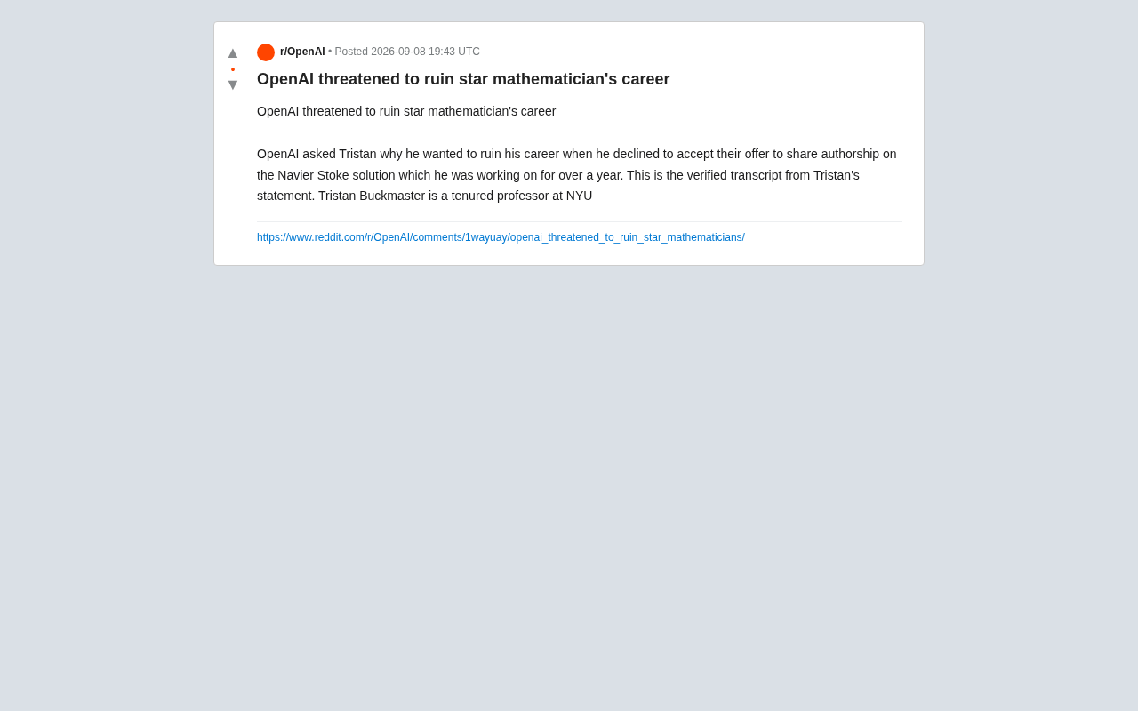
OpenAI Authorship Dispute: The Battle Over Academic Boundaries in the AI Era
OpenAI disputes authorship with mathematician Tristan Buckmaster over Navier-Stokes research, raising ethical questions about AI involvement in science.