Understand Diffusion Models in 1 Hour: From Theory to Code

Diffusion Models have become one of the core technologies in generative AI. From DALL·E 2 to Stable Diffusion, their impact has swept across the entire AI field. But many beginners are intimidated by the complex mathematical derivations and papers. Based on a hand-holding tutorial from a Bilibili creator, this article breaks down the principles, formula derivations, and code implementation of diffusion models in accessible language to help you quickly build an intuitive understanding.

From GAN to Diffusion Models: Why Do We Need a New Approach?

Generative Adversarial Networks (GANs) were once the most popular generative models, but they suffer from two major pain points: training instability and mode collapse. GANs require training a generator and a discriminator simultaneously, and the adversarial process is difficult to converge—loss functions fluctuate wildly, and the generator tends to take "shortcuts" and learn biases, resulting in poor output diversity. As the creator puts it, training a GAN is like "two players spending money to level up against each other"—ultimately one may go bankrupt while the other strikes it rich, and the process is extremely hard to control.

Diffusion models take a different path: they do not rely on adversarial training. Instead, through two processes—forward noising and reverse denoising—they gradually convert the data distribution into noise, then learn to recover data from noise. This idea was first proposed back in 2015, but it truly took off only after models like DALL·E 2 demonstrated stunning results. The creator notes that although the DALL·E 2 paper is brief, it clearly reveals its essence as being based on diffusion models.

Mode Collapse is a typical failure mode in GAN training: once the generator discovers that certain samples easily fool the discriminator, it repeatedly outputs such samples and abandons covering other modes of the data distribution. The result is highly similar generated outputs with severely insufficient diversity. For example, when trained on face data, the generator may produce only one type of face. The root cause is that the generator's goal is to "fool the discriminator" rather than "cover the true distribution"—the two objectives are not fully aligned. Diffusion models model the entire data distribution through progressive denoising, with each noise level corresponding to a learning objective, naturally avoiding this "shortcut" problem.

Forward Process: Adding Noise Step by Step Until Unrecognizable

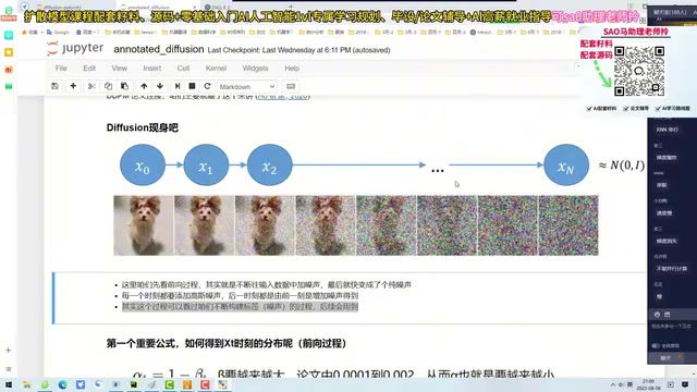
The core idea of the forward process is: gradually add Gaussian noise to the original image X0, and after T steps obtain a pure noise image XT. The amount of noise added at each step is controlled by β_t, and β_t increases over time (linearly decaying from 0.001 to 0.002), ensuring more noise is added in later stages.

Mathematically, the noising formula at each step is:

X_t = √(1-β_t) * X_{t-1} + √β_t * Z_t

where Z_t follows a standard normal distribution. Through recursion, one can derive the direct relationship between Xt at any time and X0:

X_t = √(α̅_t) * X0 + √(1-α̅_t) * Z

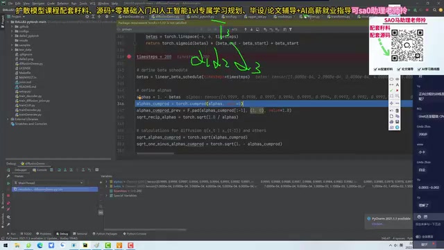
Here α_t = 1-β_t, and α̅_t is the cumulative product of α_t. The elegance of this formula lies in: no iteration needed—given X0 and t, one can directly sample Xt. The creator uses the analogy of a "drunkard walking": each step is a random offset, but the overall trend is to move further from the starting point.

The Reparameterization Trick is a key tool in deriving diffusion model formulas. When we need to sample from a Gaussian distribution N(μ, σ²), we can directly write it as μ + σ·ε, where ε follows a standard normal distribution N(0,1). This way, the sampling result's dependence on μ and σ is explicit, and gradients can flow smoothly back to the network parameters. The forward noising formula X_t = √(1-β_t)·X_{t-1} + √β_t·Z_t is exactly an embodiment of this trick: all randomness is delegated to the independent Z_t, while the mean and variance are controlled by deterministic coefficients. This allows X_t at any time to be written as a linear combination of X0 and standard noise, paving the way for deriving the closed-form solution.

Reverse Process: Recovering Data from Noise

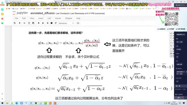
The goal of the reverse process is to gradually denoise from XT and ultimately generate X0. Directly predicting X0 from XT is almost impossible, so Bayes' formula is used to transform the problem into learning the conditional distribution p(X_{t-1}|X_t). After derivation, the mean μ_θ can be expressed as:

μ_θ = (1/√α_t) * (X_t - (β_t/√(1-α̅_t)) * ε_θ(X_t, t))

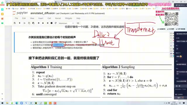
where ε_θ is a neural network used to predict noise. The creator emphasizes that this network needs X_t and time t as input (similar to Transformer positional encoding), and outputs the predicted noise. During training, the loss function is the mean squared error between the predicted noise and the true noise.

The role of Bayes' formula in the reverse process deserves elaboration. The forward process defines the known q(X_t|X_{t-1}), while the reverse process needs p(X_{t-1}|X_t)—opposite directions. Directly computing this conditional distribution requires knowing the true data distribution, which is exactly what we want to learn. Bayes' formula rewrites it as p(X_{t-1}|X_t) ∝ p(X_t|X_{t-1})·p(X_{t-1}), where the first term comes from the known Gaussian form of the forward process and the second term is approximated by a neural network. Furthermore, when β_t is sufficiently small, the conditional distribution of the reverse process can also be approximated as Gaussian, and its mean can be analytically expressed as a function of X_t and the predicted noise ε_θ—this is exactly the source of the μ_θ formula in the text.

Training and Sampling: Code in Practice

In the training phase, sample X0 from the dataset, randomly choose a time t, generate noise Z, compute Xt, then have UNet predict the noise, compute the loss, and backpropagate. The creator demonstrates using the Fashion-MNIST dataset, with code requiring only a few dozen lines. In the sampling phase, start from pure noise XT, iteratively call the trained UNet to predict noise and gradually denoise until X0 is obtained.

The creator specifically mentions that the original paper used UNet as the noise prediction network, combined with attention mechanisms. Although it remains unclear why UNet is used instead of a pure Transformer, practice shows that small-scale networks are sufficient.

Structural characteristics of UNet: UNet was originally used for medical image segmentation, and its name comes from the symmetric "U"-shaped structure—the left encoder progressively downsamples to extract semantic features, the right decoder progressively upsamples to restore spatial resolution, and skip connections directly concatenate shallow features at the same level to the decoder. In diffusion models, UNet's input is the noisy image X_t, and its output is a predicted noise map of the same size as the input. The time t is typically embedded via sinusoidal positional encoding and injected into each residual block, so the network knows which noise level it is at. Skip connections preserve high-frequency details, which is crucial for accurate noise prediction and one of the practical reasons why UNet outperforms pure Transformers.

Summary and Outlook

Diffusion models overcome many of GAN's shortcomings through a concise mathematical framework and stable training process. Although the derivation involves probability theory and the reparameterization trick, the core idea can be summarized as "adding noise is easy, denoising is hard—let a neural network help." The creator believes that diffusion models are still in a rapid development phase and may explode in more fields in the future. For beginners, it is recommended to first understand the overall process, then gradually delve into the formula details.

One-line Summary

Breaking down the forward noising, reverse denoising principles, and code implementation of diffusion models in accessible language.

Paragraph Summary

Based on a Bilibili tutorial, this article systematically organizes the core principles of diffusion models. It first contrasts the training instability and mode collapse problems of GANs, explaining that diffusion models achieve stable training through forward noising and reverse denoising. The forward process gradually adds Gaussian noise to images and can derive a closed-form relationship between Xt at any time and X0 without iteration. The reverse process uses Bayes' formula to transform denoising into learning a noise prediction network, with the loss function being the mean squared error between predicted and true noise. The noise prediction network commonly uses UNet, taking the noisy image and time t as input and outputting predicted noise. The article also provides a concise code workflow based on Fashion-MNIST and notes that diffusion models are still in rapid development, recommending beginners grasp the overall process before diving into formula details.