Why Do ResNet Skip Connections Work? Reproducing the Deep Network Degradation Problem

A Counterintuitive Experiment: Why Deep Networks Fail to Learn

A developer writing a PyTorch tutorial book wasn't content to simply tell readers that "deep plain networks perform worse" when writing the ResNet chapter. Instead, he decided to reproduce the phenomenon firsthand. He trained four networks on the CIFAR-10 dataset using an identical training recipe and random seed, with the only variables being network depth and whether skip connections were included.

CIFAR-10 is a classic image classification benchmark dataset released by Alex Krizhevsky and Geoffrey Hinton in 2009. It contains 60,000 32×32 pixel color images across 10 classes (airplane, automobile, bird, cat, deer, dog, frog, horse, ship, truck), with 50,000 for training and 10,000 for testing. While the dataset is small by today's standards with very low image resolution, these very qualities make it an ideal testbed for validating network architecture design ideas — low training cost, fast experimental turnaround, yet enough complexity to expose core issues in deep learning. The original ResNet paper also first demonstrated the degradation problem on CIFAR-10.

The brilliance of this experimental design lies in its extremely strict variable control: same recipe, same seed, same 40 epochs, eliminating virtually all confounding factors and leaving only "depth" and "residual connections" as variables.

The Degradation Problem in Numbers: Deeper Means Worse

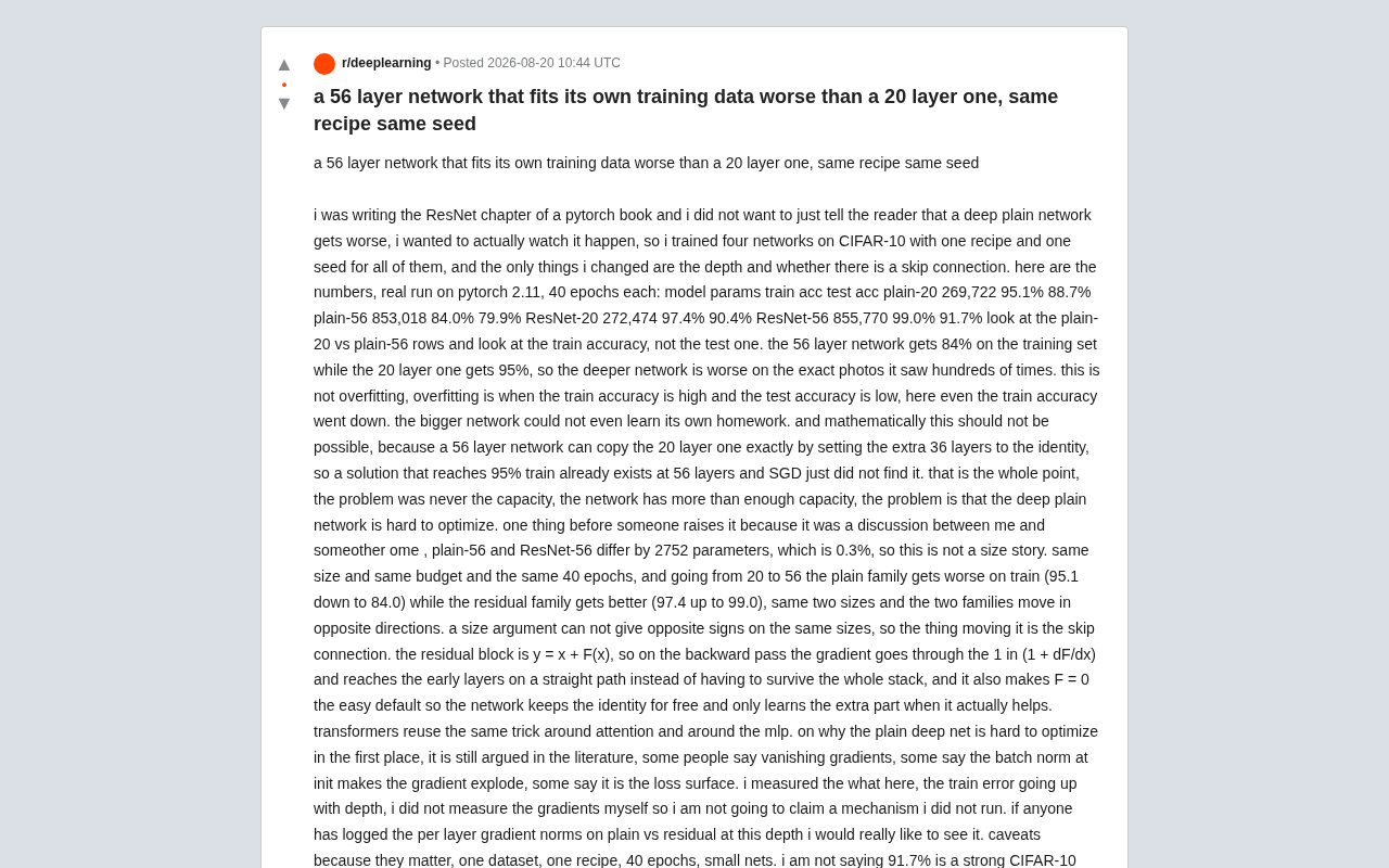
The experiment was run on PyTorch 2.11, with each model trained for 40 epochs. Here are the results:

Model	Parameters	Training Accuracy	Test Accuracy
plain-20	269,722	95.1%	88.7%
plain-56	853,018	84.0%	79.9%
ResNet-20	272,474	97.4%	90.4%
ResNet-56	855,770	99.0%	91.7%

The key point isn't the test accuracy — it's the training accuracy. Look at the plain-20 and plain-56 rows: the 56-layer plain network only achieved 84% on the training set, while the 20-layer network reached 95%. The deeper network performed worse on photos it had already "seen hundreds of times."

This is not overfitting. Overfitting is when training accuracy is high but test accuracy is low; here, the training accuracy itself dropped. As the author put it, the larger network "can't even learn its own homework." This phenomenon is a classic reproduction of the "degradation problem" identified by Kaiming He et al. in their landmark paper. ResNet (Residual Network) was proposed by Kaiming He, Xiangyu Zhang, Shaoqing Ren, and Jian Sun in 2015. Their paper Deep Residual Learning for Image Recognition won the ImageNet Large Scale Visual Recognition Challenge (ILSVRC) that year with a 3.57% Top-5 error rate, surpassing for the first time the human evaluator error rate of approximately 5.1% on ImageNet. The paper has been cited over 200,000 times, making it one of the most cited papers in deep learning history. Before ResNet, VGGNet (19 layers) and GoogLeNet (22 layers) had already begun exploring deeper networks but both hit performance saturation and even degradation bottlenecks as depth increased. He's team pushed network depth all the way to 152 layers, elegantly solving this problem through residual connections.

Why the Degradation Problem "Shouldn't" Happen Mathematically

What makes this phenomenon most puzzling is its mathematical contradiction. In theory, a 56-layer network could exactly replicate the behavior of a 20-layer network — simply by setting the extra 36 layers to identity mappings.

An identity mapping is a transformation where the input equals the output, i.e., f(x) = x. Within the theoretical framework of neural networks, the Universal Approximation Theorem tells us that a single hidden layer network with sufficient width can theoretically approximate any continuous function. Extending this to the depth dimension, deeper networks have greater function space expressiveness — this is known as network capacity. Following this logic, the solution space of a 56-layer network strictly contains that of a 20-layer network: as long as each of the extra 36 layers learns the identity mapping, the 56-layer network degenerates into a 20-layer one. However, this "constructive proof" only demonstrates the existence of a solution; it says nothing about whether the optimization algorithm can find it in finite time. This gap between "existence" and "reachability" is one of the core contradictions between theory and practice in deep learning that the degradation problem reveals.

In other words, a solution achieving 95% training accuracy already exists in the 56-layer network's parameter space — SGD simply couldn't find it.

SGD (Stochastic Gradient Descent) is the most fundamental and important optimization algorithm in deep learning. It estimates the gradient direction by randomly sampling a small batch of data at each training step, then updates parameters in the opposite direction of the gradient. However, SGD is inherently a local search algorithm — it can only see gradient information near its current position and cannot perceive the global terrain of the loss surface. The loss surface refers to the high-dimensional space formed by all possible parameter combinations and their corresponding loss values; its geometric structure determines optimization difficulty. Research has shown that the loss surfaces of deep plain networks can be riddled with "plateaus" and "saddle points," causing SGD to get trapped in suboptimal solutions and fail to find theoretically better ones. The visualization work by Li et al. in 2018 (Visualizing the Loss Landscape of Neural Nets) intuitively demonstrated how residual connections transform the loss surface from rugged and chaotic to smooth and flat, making optimization feasible.

This is the crux of the issue: the problem was never about network capacity. The network had more than enough capacity; the real obstacle is that deep plain networks are difficult to optimize. This is precisely the classic manifestation of the "degradation problem" proposed by Kaiming He et al. in the ResNet paper.

Ruling Out Model Size as a Confounding Factor

The author specifically highlighted a point that might otherwise be questioned: plain-56 and ResNet-56 differ by only 2,752 parameters, approximately 0.3%. This means the two models are nearly identical in size.

Even more compelling is the directionality of the trend: going from 20 to 56 layers, the plain network family got worse on the training set (95.1% → 84.0%), while the residual network family got better (97.4% → 99.0%). Same two scales, but the two families moved in opposite directions.

The author put it incisively: "A scale argument cannot produce opposite signs at the same scale." Since the scales are identical yet the results are opposite, the only thing that could be making the difference is the skip connection.

How ResNet Skip Connections Work

The residual block formula is y = x + F(x). This seemingly simple structure brings two key advantages:

A "Highway" for Gradient Backpropagation

During backpropagation, gradients pass through the "1" in (1 + dF/dx), reaching early layers via a direct path rather than having to "survive" layer-by-layer attenuation through the entire network stack. The residual connection provides a shortcut for gradient flow that never vanishes.

To understand why this matters, you need to know about vanishing gradients and exploding gradients — two classic pathological phenomena in deep network training. During backpropagation, gradients must be multiplied layer by layer through the chain rule. If each layer's gradient multiplier is slightly less than 1, after dozens of layers of accumulation the gradient decays exponentially toward zero, leaving early layers virtually unable to update — this is vanishing gradients. Conversely, if the multiplier is slightly greater than 1, gradients grow exponentially — this is exploding gradients. Although BatchNorm (Batch Normalization, proposed by Ioffe and Szegedy in 2015) partially alleviates both problems by normalizing each layer's output to stabilize the numerical range of gradients, some research (such as Yang et al., 2019) has pointed out that BatchNorm may actually introduce new gradient instabilities during early training, which means the root cause of the degradation problem remains debated to this day. The constant "1" in residual connections provides a propagation channel unaffected by network depth, fundamentally bypassing this dilemma.

Identity Mapping as the Default Solution

The residual structure makes F = 0 a cheap default option. The network can "freely" preserve the identity mapping, only learning additional transformations when they actually help. This fundamentally solves the optimization dilemma mentioned earlier where "SGD can't find the identity solution." From an optimization perspective, getting a network layer composed of convolutional layers and nonlinear activation functions to learn a precise identity mapping is surprisingly difficult — the network would need to adjust all weights to specific values exactly. But in a residual structure, the identity mapping comes "for free": as long as the weights of F(x) are close to zero, the entire residual block automatically degenerates into an identity mapping. This means that by default, extra layers cause no harm; the network only needs to learn "how much correction to make on top of the identity mapping" rather than learning the entire transformation from scratch.

It's worth noting that the Transformer architecture reuses this exact same trick around both attention mechanisms and MLPs — residual connections have long become indispensable infrastructure in modern deep learning architectures. The Transformer architecture proposed by Vaswani et al. in 2017 (paper Attention Is All You Need) uses residual connections combined with Layer Normalization around every sub-layer (self-attention and feed-forward network layers), i.e., output = LayerNorm(x + Sublayer(x)). In modern large language models like GPT, BERT, and LLaMA, model depth routinely reaches dozens or even hundreds of Transformer blocks — without residual connections, these models simply couldn't be trained. In fact, improvements around residual connections remain actively pursued in recent years. For example, the choice between Pre-Norm (placing LayerNorm before the sub-layer) and Post-Norm, and DeepNorm (a deep Transformer stable training scheme proposed by Microsoft) all demonstrate that the specific implementation of residual connections still has profound implications for the trainability of ultra-deep networks.

Honest Scientific Attitude: Measuring "What" Rather Than "Why"

Regarding why deep plain networks are difficult to optimize, the author displayed a commendably rigorous attitude. He candidly acknowledged that this remains debated in academia: some attribute it to vanishing gradients, others believe it's due to gradient explosion caused by BatchNorm during initialization, and still others point to the geometric structure of the loss surface.

The author explicitly stated: "What I measured here is the 'what' — the phenomenon that training error increases with depth. I didn't personally measure gradients, so I won't claim a mechanism I haven't verified myself." He even publicly solicited contributions, hoping someone could share per-layer gradient norm logs for plain networks versus residual networks at these depths.

This attitude of distinguishing between "phenomenon" and "mechanism" is especially precious in deep learning research. The field is rife with "post-hoc explanations" — constructing seemingly plausible theoretical explanations after observing experimental results that may not withstand rigorous verification. For example, the explanation for why BatchNorm works has undergone a paradigm shift from "reducing internal covariate shift" to "smoothing the loss surface." The author's choice to only report data he personally measured, without making inferences beyond the evidence, is precisely the most reliable scientific method.

Experimental Limitations and Open Discussion

The author also honestly listed the experiment's caveats: a single dataset (CIFAR-10), a single recipe, 40 epochs, small-scale networks. He emphasized that 91.7% is not the best result achievable on CIFAR-10 — tuned networks can go much higher. His claim is limited to "the directional difference between two network families under identical training conditions."

Finally, he posed open questions to the community: Has anyone seen cases where the degradation phenomenon doesn't appear? For instance, a certain depth at which plain networks stop getting worse, or a training recipe that fixes degradation without relying on skip connections?

These questions are not without precedent. For example, some researchers have found that specific initialization schemes (such as LSUV, Layer-Sequential Unit-Variance initialization) or particular normalization strategies can mitigate the degradation problem to some extent. Additionally, NFNet (Normalizer-Free Networks), proposed in 2020, demonstrated the possibility of training very deep networks without BatchNorm through carefully designed initialization and adaptive gradient clipping — but notably, NFNet still relies on residual connections. These follow-up works indirectly confirm both the complexity of the degradation problem and the irreplaceability of residual connections.

This spirit of "reproducing classics firsthand and honestly acknowledging the boundaries of the unknown" is the most admirable attitude in technical writing. It transforms a textbook conclusion back into an observable, verifiable scientific question that still deserves deeper investigation.

Key Takeaways