Deep Learning Lane Detection: From Segmentation to Classification for 300+ FPS Real-Time Inference

Introduction: Why Does Lane Detection Need Deep Learning?

When it comes to lane detection, many people's first thought is that a few lines of OpenCV code can get the job done. Indeed, traditional methods can achieve basic lane line recognition, but in real-world driving scenarios, the challenges go far beyond that: vehicle occlusion, lighting changes, worn lane markings, degraded accuracy at long distances... These problems leave traditional methods struggling.

Traditional lane detection typically relies on classic image processing algorithms like Canny edge detection and Hough Transform. The basic pipeline is: convert the image to grayscale, apply Gaussian blur for noise reduction, extract edges with the Canny operator, and finally fit lines using the Hough Transform. This pipeline works well under ideal conditions with uniform lighting and clear lane markings, but it fundamentally depends on hand-crafted features and fixed threshold parameters. Once you encounter shadows, backlighting, rain/snow, or faded lane markings, these fixed thresholds fail across the board. Moreover, traditional methods struggle with curved lanes (Hough Transform can only detect straight lines) and cannot distinguish between different types of lane markings. Deep learning methods, through end-to-end feature learning, can automatically adapt to various complex scenarios — this is their fundamental advantage over traditional approaches.

The algorithm introduced today is a deep learning-based lane detection method whose core idea is simplifying dense segmentation into efficient classification, achieving 300+ FPS real-time inference speed while maintaining detection quality. This approach holds tremendous engineering value for practical scenarios requiring deployment on in-vehicle devices.

Lane Detection Dataset and Data Processing Pipeline

Dataset: Collected from Real Roads in Beijing

This algorithm uses an academic research dataset collected from real road scenarios in Beijing, which can serve as a benchmark for domestic lane detection. The dataset covers various road conditions: streets of different widths, pedestrian-dense areas, heavily occluded scenarios, etc., providing excellent representativeness.

It's worth noting that the complete dataset is very large — a single video can be several hundred megabytes, and the entire dataset easily reaches tens or even hundreds of gigabytes. For learning and experimentation, a streamlined demo dataset can be used to run through the entire pipeline.

Data Augmentation Strategy

Given the characteristics of lane detection tasks, data augmentation primarily employs two approaches:

• Extensive translation operations: This is the most effective augmentation method, simulating scenarios where the vehicle drives in different lane positions
• Small-angle rotations: Note the emphasis on "small-angle" — in reality, lane lines cannot appear in the sky, and excessive rotation would introduce unreasonable samples

Label Extension Processing

Public datasets commonly have an annotation issue: labels are intermittent, especially for distant lane markings where annotations are frequently missing. The algorithm addresses this with a linear fitting extension method — extending labels into the distance based on the trend of existing annotation points. This is reasonable because from the driver's perspective, even with curves, lane lines are approximately straight within a local range.

Core Algorithm Concept: From Dense Segmentation to Efficient Classification

Why Not Use Semantic Segmentation Directly?

Lane detection is essentially a semantic segmentation task — determining whether each pixel in the image belongs to a lane line. But segmentation methods have a fatal problem: the computational cost is too high.

Semantic segmentation is one of the fundamental tasks in computer vision, aiming to assign a class label to every pixel in an image. Since FCN (Fully Convolutional Network) pioneered the replacement of fully connected layers with convolutional layers in 2015, semantic segmentation has evolved through multiple architectural generations including SegNet, U-Net, and the DeepLab series. In autonomous driving, semantic segmentation is widely used for road area recognition and drivable area detection. However, the computational overhead of per-pixel prediction is enormous — even lightweight segmentation networks struggle to meet real-time requirements with high-resolution inputs. Particularly on in-vehicle embedded platforms (such as the NVIDIA Jetson series), both computational power and power consumption are strictly limited, motivating researchers to explore more efficient alternatives.

Take a 300×800 image as an example: segmentation requires prediction at 300×800 = 240,000 positions, multiplied by 4 lane lines, ultimately outputting a 300×800×4 matrix. Such computational demands make real-time processing on in-vehicle devices extremely difficult.

Key Simplification: Row Selection + Grid Classification

The core innovation of this paper lies in simplifying both the H and W dimensions:

H dimension (row direction) simplification: Only 18 key rows are selected from 300 rows as prior positions. The selection of these 18 rows is based on statistical characteristics of the dataset and is a manually specified hyperparameter. Why only 18? Because lane lines don't change abruptly — 18 sampling points are sufficient to describe the trajectory of a lane line.

W dimension (column direction) simplification: Each row is divided into 200 grid cells, and then a 200-class classification is performed — predicting which grid cell the lane line falls on.

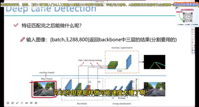
This way, the original 300×800 dense prediction is simplified to an 18×200 sparse prediction, dramatically reducing computational cost. The final model output is a 201×18×4 tensor:

• 4: 4 lane lines
• 18: 18 key rows for each lane line
• 201: 200 grid positions + 1 "no lane line exists" class

Auxiliary Segmentation Branch: Multi-Task Learning for Better Features

The network architecture in the paper contains two branches: the segmentation branch on top and the lane classification branch below. There's an elegant design principle here — the segmentation branch is only used during training and completely removed during testing.

Here's an analogy: it's like playing a video game where your goal is to become the strongest mid-laner, but during practice you also train as a jungler because jungling improves your fundamental mechanics. Similarly, simultaneously performing segmentation during training helps the backbone extract better features, indirectly improving lane detection performance. But during actual inference, only the classification branch is used, with no impact on inference speed.

The theoretical foundation of Multi-Task Learning (MTL) dates back to Rich Caruana's classic 1997 paper. Its core hypothesis is that related tasks share underlying feature representations, and joint training can serve as implicit data augmentation and regularization. From an optimization perspective, auxiliary tasks provide additional gradient signals for the main task, helping shared layers learn more generalizable features. In the deep learning era, this concept has been widely applied: Mask R-CNN simultaneously optimizes bounding box regression, classification, and instance segmentation; MTCNN simultaneously predicts face boxes and keypoints in face detection. The design of the segmentation branch as an auxiliary task in this paper is particularly clever — it provides pixel-level supervision during training, forcing the backbone to learn finer spatial features, but is completely removed during inference, adding zero computational overhead. This "complex during training, simple during inference" strategy is a highly practical technique in engineering deployment.

Loss Function Design: Triple Constraints for Detection Quality

Another highlight of this algorithm is its carefully designed loss function system, comprising three components:

Focal Loss: Addressing Positive-Negative Sample Imbalance

Determining which grid cell a lane line occupies is essentially a classification problem. Due to severe positive-negative sample imbalance (only a few out of 200 grid cells contain lane lines), Focal Loss is used to balance sample weights — a classic approach for handling class imbalance.

Focal Loss was proposed by Kaiming He et al. in the 2017 RetinaNet paper, originally designed to address the extreme foreground-background sample imbalance in object detection. Its core idea is to introduce a modulating factor (1-p_t)^γ on top of standard cross-entropy loss, where p_t is the model's predicted probability for the correct class and γ is a tunable focusing parameter (typically set to 2). When the model already has high confidence for a sample, the modulating factor approaches 0, greatly reducing that sample's contribution to the loss; for hard-to-classify samples, the modulating factor stays close to 1, keeping the loss unchanged. This way, training attention automatically focuses on hard samples. In lane line grid classification, there may be only 1-2 positive samples among 200 grid cells, and Focal Loss effectively prevents the large number of negative samples from dominating gradient updates, thereby improving the model's discriminative accuracy for lane line positions.

Similarity Loss: Adjacent Point Consistency Constraint

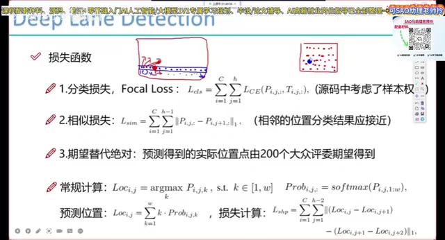
An important prior for lane lines is: predictions for adjacent points should be similar. If a point is predicted as a lane line, its neighboring points above and below are very likely also lane lines; and vice versa. The similarity loss constrains that prediction probabilities for the same lane line on adjacent rows should be close, preventing the model from predicting unreasonable "sharp turns."

Shape Loss: Second-Order Smoothness Constraint

The shape loss goes further — it not only requires small differences between adjacent pairs of points but also requires that the pairwise differences among three consecutive points should be similar. This acts as a second-order smoothness constraint, ensuring that the predicted lane line is smooth and continuous in its overall shape.

Expectation-Based Localization: Weighted Voting Instead of Hard Classification

When determining the final lane line position, the algorithm doesn't simply take the grid cell with the highest probability. Instead, it computes a weighted expectation across all grid cells' predictions. Each grid cell acts like a "jury member," voting on the final position according to its predicted probability. This expectation-based localization is more robust than argmax and significantly improves the model's generalization ability — this shares the same philosophy as SenseTime's approach in keypoint detection.

Expectation-based Localization originates from Integral Regression, first proposed by Jian Sun's team at SenseTime for human pose estimation. Traditional keypoint detection methods use argmax to take the position with the highest probability from a heatmap as the prediction, but argmax is non-differentiable, cannot be trained end-to-end, and is sensitive to noise. Integral regression treats the heatmap as a probability distribution and obtains continuous coordinate predictions through probability-weighted summation of all position coordinates (i.e., mathematical expectation). This method is not only differentiable but also inherently smooth — even if the heatmap has multiple local peaks, the expected value provides a reasonable compromise position. In this paper's lane detection, computing the weighted expectation over softmax probabilities of 200 grid cells is essentially an application of this concept, enabling final lane line position predictions to break through the quantization error introduced by grid discretization.

Practical Results and Engineering Deployment

Performance: 300+ FPS Real-Time Inference

This algorithm achieves 300+ FPS inference speed while maintaining detection accuracy, and the hardware used is not high-end. This means it is fully capable of running in real-time on in-vehicle embedded devices.

In challenging scenarios such as occlusion, long distance, and worn lane markings, the algorithm still delivers good predictions, thanks to:

• Prior row selection reducing noise interference
• Structural losses ensuring prediction smoothness
• Expectation-based localization improving robustness

Deployment Path: From Server to Edge Devices

For engineering deployment, there are two main paths:

• Server deployment: Based on Docker + Flask, relatively straightforward
• Edge device deployment: Deploying to embedded devices through the ONNX → TensorRT conversion pipeline — this is the mainstream approach for actual in-vehicle scenarios

ONNX (Open Neural Network Exchange) is an open neural network interchange format jointly launched by Microsoft and Facebook in 2017, designed to enable model interoperability between different deep learning frameworks. By exporting models trained in PyTorch or TensorFlow to ONNX format, they can run on different inference engines. TensorRT is NVIDIA's high-performance deep learning inference optimizer and runtime library, deeply optimized specifically for NVIDIA GPUs. TensorRT's core optimization techniques include: layer fusion (merging multiple network layers into a single kernel execution), precision calibration (supporting FP16 and INT8 quantization for significantly improved throughput with controllable accuracy loss), dynamic tensor memory management, and automatic kernel tuning for specific GPU architectures. The complete deployment pipeline is typically: PyTorch model → ONNX intermediate representation → TensorRT engine (.engine file) → embedded device inference. On automotive-grade platforms like NVIDIA Jetson Xavier NX, TensorRT-optimized models typically achieve 3-5x inference acceleration.

Summary: Balancing Speed and Accuracy

The core insight from this paper is: algorithm optimization isn't just about pursuing higher accuracy — reducing computational cost is equally important as a research direction. By simplifying dense segmentation into sparse classification, combined with carefully designed loss functions, the algorithm achieves an excellent balance between speed and accuracy.

For those looking to get started in autonomous driving perception, this project is an excellent starting point: the algorithmic concept is clear, the code is runnable, and the engineering value is evident — it can absolutely serve as a highlight project on your resume.

Key Takeaways