CPU Inference Optimization in Practice: Quantization, SetFit, and Conformal Prediction Workshop

When Decision Systems Must Run on CPU

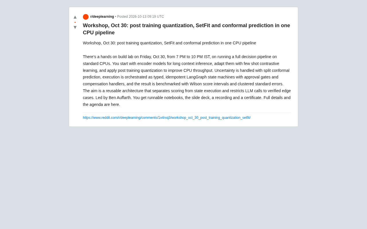
Discussions about large model inference tend to revolve around GPUs, but in real enterprise environments, many decision pipelines ultimately still have to run on standard CPUs—not because there's no desire to use GPUs, but because cost, deployment environment, and latency constraints all point in that direction. A hands-on workshop preview appeared on Reddit around this problem: running a complete decision pipeline on standard CPUs, starting from long-context inference with encoder models, passing through few-shot contrastive learning adaptation, then using post-training quantization to improve throughput, and finally applying conformal prediction to handle uncertainty.

The workshop is scheduled for Friday evening from 7 to 10 PM (IST), led by Ben Auffarth, and includes runnable notebooks, slides, recordings, and certificates. The technology stack is quite comprehensive and worth breaking down.

The Synergistic Logic of Three Technical Pillars

Post-Training Quantization: Unlocking Throughput from the Bottleneck

When encoder models perform long-context inference, memory bandwidth and compute on the CPU are both hard constraints. Post-training quantization compresses model weight precision without retraining, directly reducing memory usage and computation. The value of this path lies in its low engineering cost—no need for labeled data to flow back, and no need for gradient updates, so it can be applied directly to models already in production.

The difficulty lies in controlling accuracy loss after quantization. Encoder-type models are usually more sensitive to numerical precision in attention layers than in FFN layers, so quantization strategies need to be layer-specific rather than one-size-fits-all. This is also what makes the hands-on portion of the workshop worth watching.

Post-Training Quantization (PTQ) is one of the major categories of model compression alongside Quantization-Aware Training (QAT): QAT inserts fake quantization nodes before training so the model adapts to low-precision representations during training; PTQ directly performs numerical mapping on trained weights without backpropagation. Common mapping methods include symmetric quantization, which maps a floating-point interval symmetrically to an integer range, and asymmetric quantization, which introduces a zero-point offset for data not centered at zero. On CPU, low-bit weights can directly reduce memory bandwidth pressure and enable inference through int8 or narrower bit-width vectorized instructions (such as AVX-VNNI). An empirical rule for encoder models is that attention layers have a larger dynamic range in their weights, and aggressive quantization can easily distort attention distributions, while FFN layers are usually more robust. Therefore, mixed-precision strategies are often used in practice, retaining higher bit-width for some tensors in attention layers, or using per-channel quantization instead of per-tensor quantization to mitigate error.

SetFit: Contrastive Learning Adaptation in Few-Shot Scenarios

SetFit works by first using a small number of labeled samples for contrastive learning, then training a classification head. Compared with directly fine-tuning a large model, it has a clear advantage in sample efficiency, and its training cost is low—which fits precisely with the overall positioning of a CPU pipeline.

Whether SetFit is placed before or after quantization directly affects final accuracy. Adapt first and then quantize, and quantization error acts on the decision boundary that has already been learned; quantize first and then adapt, and the contrastive learning stage may fail to learn effective representations because of precision loss. The order of the workshop pipeline is worth noting.

The key mechanism behind SetFit is contrastive learning at the sentence embedding level, rather than direct fine-tuning at the model output layer. It first uses a small number of labeled samples to construct positive and negative pairs, pulls embeddings of similar samples closer and pushes embeddings of dissimilar samples farther apart through a contrastive loss, and then trains a lightweight classification head on these adapted embeddings. Positive pairs usually come from a positive example of the same sample and other samples of the same class, and can be expanded through data augmentation, so very few samples per class are enough to form an effective gradient signal. Compared with prompt engineering or full-parameter fine-tuning, SetFit limits learnable parameters to a very small range, significantly reducing training epochs and memory requirements, making it suitable for rapid iteration on constrained hardware. The tradeoff is that it depends on the quality of the pretrained embeddings themselves: if the base encoder is too far from the target domain, the room contrastive learning can move is limited, and domain adaptation must be done first.

Conformal Prediction: Adding Quantifiable Uncertainty to Decisions

The core value of split conformal prediction is providing prediction intervals or prediction sets with statistical guarantees. In a decision pipeline, this means the system can output "how certain I am" rather than just a label.

In practical deployment, conformal prediction requires a calibration set to estimate quantiles, and distribution shift in the calibration set directly breaks the theoretical guarantee of coverage. When combining it with a quantized model, calibration must be performed on the quantized model—using the pre-quantization model for calibration will invalidate the coverage guarantee. This is an easily overlooked detail with serious consequences.

The core of split conformal prediction is constructing a conformity score, for example in classification tasks commonly using 1 minus the predicted probability of the true class. Compute the scores of all samples on the calibration set and take their empirical quantile to obtain a threshold; at inference time, include all candidate classes whose scores do not exceed that threshold in the prediction set. The theoretical guarantee is this: under the assumption of exchangeability of the data, the prediction set covers the true label with probability at least 1-α, where α is a preset significance level. This guarantee is non-asymptotic and does not depend on model form or data distribution, only on the calibration set and test set coming from the same distribution. Therefore, when distribution drift exists, coverage fails, and recalibration on the target distribution is needed. In addition, the smaller the calibration set, the less stable the quantile estimate, and the actual coverage will deviate from the nominal value, requiring a tradeoff between sample size and guarantee strength. Conformal prediction can also output prediction intervals for regression tasks by simply replacing the score definition, such as absolute residual.

LangGraph State Machine: Separating Scoring from Execution

In the architecture proposed by the workshop, the execution layer uses LangGraph to build typed, idempotent state machines with approval gates and compensation handlers. The core intent of this design is to separate scoring from state execution and limit LLM calls to validated edge cases.

Idempotency in a state machine means retries do not produce side effects, while compensation handlers correspond to transaction rollback in the Saga pattern. The presence of approval gates indicates that the pipeline is aimed at decision scenarios requiring human intervention—not fully automated batch processing, but a process with human review nodes.

Limiting LLM calls to edge cases is essentially a cost-control strategy: most inputs are handled by lightweight encoder models, and only low-confidence or out-of-distribution samples trigger more expensive LLM calls. Conformal prediction plays the role of a router here—samples whose prediction set is too large or whose uncertainty is too high are sent to the LLM.

Why Benchmarking Uses Wilson Intervals and Clustered Standard Errors

The workshop uses Wilson score intervals and clustered standard errors for benchmarking, a choice far more rigorous than simply reporting accuracy.

The Wilson interval is suitable for estimating binary proportions and is more reliable than the normal approximation in small samples. Clustered standard errors address correlation among samples—if the test data contains multiple samples from the same source or same user, the i.i.d. assumption is broken, and ordinary standard errors will be underestimated. Using these two tools together shows that the workshop has requirements for statistical rigor in evaluation.

When evaluating classification performance, using point estimates such as accuracy or recall directly can easily ignore uncertainty. The Wilson score interval shrinks the observed proportion toward 0.5 and adjusts the standard error, so that even when the sample size is small or the proportion is close to 0 or 1, the interval still lies within [0,1] and has reasonable coverage, whereas the ordinary normal approximation gives out-of-bounds intervals at extreme proportions. Clustered standard errors address the case of non-independent samples: if data are grouped by user, session, or document, samples within the same group are correlated, and treating each sample as an independent observation underestimates variance. In this case, one should first aggregate within groups to obtain group-level statistics, then compute standard errors using the number of groups as the sample size, or use cluster-robust variance estimation. Combining these two methods makes benchmark reports carry more credible error ranges and also makes it easier to compare whether differences between pipelines truly exceed noise.

Who This Pipeline Is For

If your scenario meets the following conditions, this architecture is worth investing time to study: decision latency requirements within what the CPU can bear, limited labeled samples, the need for interpretable uncertainty outputs, and human review nodes in the process.

Less suitable scenarios: real-time inference requiring extremely high throughput, or tasks whose accuracy requirements approach the upper limit of GPU fine-tuning. The positioning of a CPU pipeline is to find a balance between cost and availability, not to pursue absolute performance.

Key Takeaways

• Post-training quantization significantly improves encoder model throughput on CPU, but layer-specific quantization strategies are needed to control accuracy loss
• SetFit's few-shot contrastive learning reduces adaptation cost, and its order relative to quantization affects the final result
• Split conformal prediction provides uncertainty outputs with statistical guarantees, and calibration must be performed on the quantized model
• The LangGraph state machine achieves idempotent execution through approval gates and compensation handlers, with LLM calls limited to low-confidence edge cases
• Evaluation methods using Wilson intervals and clustered standard errors reflect true performance better than simple accuracy

The specific technical details of the workshop will need to be verified after the notebook and recording are released, but the design approach at the architecture level is already clear enough: running a decision pipeline on CPU depends not on the performance of a single model, but on how the four layers—quantization, few-shot adaptation, uncertainty quantification, and state orchestration—work together.

One-line Summary

Building a decision pipeline on standard CPUs requires four layers working together: quantization, few-shot adaptation, conformal prediction, and state orchestration.

Paragraph Summary

The article centers on a hands-on workshop for running a complete decision pipeline on standard CPUs and introduces the synergistic logic of four key technologies. Post-training quantization improves throughput by compressing encoder model weights, but layer-specific quantization strategies are needed to control accuracy loss; SetFit uses a small number of labeled samples for contrastive learning adaptation, and its order relative to quantization directly affects the final result; split conformal prediction provides uncertainty outputs with statistical guarantees, but calibration must be performed on the quantized model, otherwise the coverage guarantee fails. The execution layer uses LangGraph to build idempotent state machines with approval gates and compensation handlers, limiting LLM calls to low-confidence or out-of-distribution edge cases, essentially a cost-control strategy. For evaluation, Wilson score intervals and clustered standard errors are used, which is more rigorous than simply reporting accuracy. The article concludes that this architecture is suitable for scenarios with controllable latency, limited labeled samples, a need for uncertainty outputs, and human review nodes, and unsuitable for tasks pursuing extremely high throughput or accuracy approaching the upper limit of GPU fine-tuning.