How to Quantify Image Size and Shape Changes After Data Augmentation?
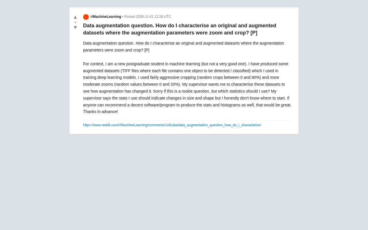
Quantify the impact of crop and scale augmentation on dataset distribution using size and shape statistical metrics
The article addresses a machine learning graduate student asked by his advisor to quantify the impact of random cropping (0–90%) and random scaling (0–20%) on image targets, pointing out that the core question is whether the augmented dataset distribution still represents the original distribution or has introduced measurable bias. The author recommends two dimensions: size (mean, standard deviation, median, and IQR of bounding box width, height, and area, with histograms or KDE curves comparing original and augmented distributions) and shape (aspect ratio distribution as the primary metric, supplemented by circularity and other shape factors, plus cross analysis binned by original size to observe asymmetric effects on small versus large targets). The Python ecosystem (scikit-image, OpenCV, pandas, matplotlib, tifffile for TIFF) is recommended, with the pipeline written as a reusable script. Finally, it reminds to record sampled augmentation parameters and combine parameter distribution with result distribution to fully answer how, to what extent, and in which direction augmentation changes the data.
A machine learning graduate student generated an augmented dataset using random cropping (0–90%) and random scaling (0–20%), and his advisor asked him to quantify the impact of these augmentations on image size and shape. This question is fairly representative in practice—the effects of data augmentation are often judged by feel, lacking interpretable statistical descriptions.
The Essence of the Problem: What Augmentation Changes
The student's scenario is specific: each TIFF file contains a target to be detected or classified. After random cropping and scaling, the target's proportion in the image, bounding box size, and aspect ratio may all undergo systematic shifts. The advisor's request actually points to a core question: does the augmented dataset distribution still represent the true distribution of the original data, or has it introduced measurable bias?
Cropping directly removes edge regions. When the crop ratio reaches 90%, some targets may be partially truncated or completely lost. Although scaling is mild (0–20%), it changes the absolute size of targets in pixel space. After combining both, the statistical characteristics of the augmented dataset in the two dimensions of "size" and "shape" need to be explicitly characterized; otherwise, subsequent changes in model performance will be difficult to attribute.
Statistical Metrics for the Size Dimension
For size changes, the most direct measures are the width, height, and area of the target bounding box. It is recommended to calculate the mean, standard deviation, median, and interquartile range of these quantities for both the original and augmented datasets, and to plot distribution histograms or kernel density estimation curves for comparison.
If each file in the dataset contains only one target, the target region can be extracted via connected component analysis or simple threshold segmentation, and then the bounding rectangle can be computed. For data already annotated with bounding boxes, the annotation boxes can be used directly. The key is not how complex the statistics are, but to visually compare the two distributions—original and augmented—in the same coordinate system: mean shift reflects systematic scaling, while variance change reflects the degree of randomness introduced by augmentation.
One easily overlooked point: when cropping to 90%, many samples may retain only a small region, and the area distribution may exhibit a long tail or even zero values. Such samples should be marked separately in the statistics because their contribution to detection tasks differs from that of traditional samples.
Connected component analysis is a fundamental operation in binary image processing: adjacent pixels of the same class (usually foreground pixels) are aggregated into independent regions, each being a connected component. In target extraction scenarios, a foreground mask is first obtained via threshold segmentation, then connected component labeling is applied to the mask to separate individual targets and compute their bounding boxes. Common implementations include scikit-image's measure.label and regionprops, and OpenCV's connectedComponentsWithStats. Note that the difference between 4-connectivity and 8-connectivity definitions affects the merging of small regions, and is especially sensitive for elongated or diagonally adjacent targets.
Interquartile Range (IQR) is the difference between the third quartile and the first quartile, i.e., the spread of the middle 50% of the data. Compared with standard deviation, IQR is insensitive to extreme values, making it particularly suitable for describing target area distributions that may have long tails or even zero values after cropping. When augmentation causes some sample targets to nearly disappear, the standard deviation will be significantly inflated by these outliers, while IQR still robustly reflects the dispersion of the main body of samples. In practice, it is often used with box plots, where the top and bottom edges of the box correspond to Q1 and Q3.
Methods for Characterizing the Shape Dimension
Shape changes are more subtle than size. Both cropping and scaling can alter the aspect ratio of targets, especially when targets are non-square. Comparing the distribution of aspect ratios is the first step, which can intuitively show whether augmentation makes targets more "slender" or more "squat".
If richer shape descriptions are needed, shape factors (such as circularity, compactness) or contour-based moment features can be introduced. However, for the advisor's requirement to "indicate size and shape changes", the joint distribution of aspect ratio plus bounding box size is usually sufficient. More complex shape descriptors may be over-engineering for a preliminary analysis at the graduate level, and may instead increase the cost of interpretation.
Cross analysis is also worth doing: bin samples by original size and observe the magnitude of size change after augmentation within each bin. This can reveal whether the impact of augmentation is symmetric for small and large targets.
Circularity is defined as $4\pi A / P^2$, where $A$ is the region area and $P$ is the perimeter. It ranges from 0 to 1, with values closer to 1 indicating shapes closer to a circle. Compactness is often expressed as $P^2 / A$ or its normalized form, which is the reciprocal of circularity; larger values indicate more irregular shapes or more complex boundaries. Both are sensitive to boundary noise and segmentation quality, so when comparing before and after augmentation, the segmentation or annotation pipeline should be kept consistent; otherwise, the measured differences may come from the extraction method rather than the augmentation itself.
Tool Selection and Practical Advice
The student asked about specific software. The Python ecosystem is the most direct choice: use scikit-image or OpenCV for region extraction and contour analysis, pandas for organizing statistical tables, and matplotlib or seaborn for histograms and violin plots. If the data already has annotations in COCO or YOLO format, pycocotools or direct parsing of label files can provide bounding boxes.
TIFF files require extra attention to bit depth and number of channels; using the tifffile library is more reliable than general-purpose image libraries for reading them. It is recommended to write the statistical pipeline as a reusable script: input the original directory and augmented directory, output comparison statistical tables and distribution plots, so that the advisor can review or rerun directly when adjusting augmentation parameters later.
A Practical Reminder
If the augmentation parameters themselves (the actual sampled values of crop ratio and scaling factor) can be recorded in metadata at generation time, subsequent analysis will be much easier. If they were not recorded, they can also be partially inferred from the size differences between before and after images. Either way, only by looking at the "parameter distribution" together with the "result distribution" can the advisor's question be fully answered: to what extent and in which direction does augmentation change the dataset.
One-line Summary
Quantify the impact of crop and scale augmentation on dataset distribution using two-dimensional statistical metrics of size and shape
Paragraph Summary
The article addresses a scenario where a machine learning graduate student is asked by his advisor to quantify the impact of random cropping (0–90%) and random scaling (0–20%) on image targets. It points out that the core question is whether the augmented dataset distribution still represents the original distribution or has introduced measurable bias. The author suggests proceeding from two dimensions: size and shape. For size, calculate the mean, standard deviation, median, and interquartile range of bounding box width, height, and area, and plot histograms or kernel density curves to compare original and augmented distributions. For shape, use aspect ratio distribution as the primary metric, supplemented by shape factors such as circularity, and observe asymmetric effects on small versus large targets through cross analysis binned by original size. At the tool level, the Python ecosystem is recommended (scikit-image, OpenCV, pandas, matplotlib, tifffile for TIFF), and the pipeline should be written as a reusable script. Finally, it reminds to record the sampled values of augmentation parameters and combine parameter distribution with result distribution to fully answer how, to what extent, and in which direction augmentation changes the data.
Related articles
GitHub Daily · November 05: Skills Ecosystem Explodes, Agents Begin to Take Over the Desktop
GitHub Daily Nov 5: Skills ecosystem explodes with five 'skills' repos trending; vercel-labs' agent-desktop and agent-browser build agent limbs; Rust dominates agent infrastructure.

Deleted Reddit Post Sparks Debate Over AI Content Moderation
A Reddit post removed with only a 'Removed by Reddit' notice highlights AI content moderation's transparency gaps, misjudgment risks, and appeal challenges for platforms and creators.

DSH + Ollama Local LLM Deployment in Practice: Free Chat with Da Fei Yu
Bilibili creator tests DSH + Ollama local LLM deployment end to end: Ollama install, Xunlei-accelerated downloads, ModelScope GGUF model import, DSH custom API address setup, and a comparison of Qwen 3.5 4B, 8B, Gemma, and other models on 8GB VRAM, with advice on choosing local deployment vs. API calls.