Rainbow DQN Has No New Ideas: A Complete Guide to the Evolution of Value-Based Reinforcement Learning Algorithms

A Counterintuitive Starting Point: Rainbow Has No New Ideas

In the history of reinforcement learning, Rainbow is often regarded as the magnum opus of value-based methods. But a developer shared an interactive tutorial on Reddit that offers a counterintuitive yet precise insight: Rainbow didn't invent anything new. It simply "turned on" six previously existing improvement patches simultaneously and observed their combined effect.

This perspective is valuable because it reinterprets the famous ablation table in the Rainbow paper as a "tutorial table of contents"—each component whose removal causes performance degradation corresponds to a critical fix in DQN's evolutionary history. Understanding Rainbow essentially means understanding what problem each of these six fixes solved.

The ablation experiment in the Rainbow paper (Hessel et al., 2018) carries methodological significance beyond mere engineering validation. The experimental design uses all six components enabled simultaneously as the baseline (rather than starting from vanilla DQN and adding components one by one), removing one component at a time and observing the performance drop. This "subtractive ablation" reveals each component's marginal contribution and the synergies between components. Results show that removing prioritized experience replay and removing distributional learning cause the most damage, while removing the dueling architecture has relatively less impact. Notably, the combined effect of all six components significantly exceeds the sum of any individual component's contribution, suggesting positive interactions between components—for example, the more precise TD errors produced by distributional learning happen to provide better priority signals for prioritized experience replay.

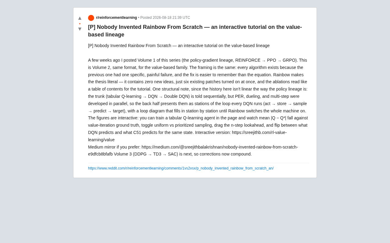
This is the second volume of the tutorial series. The author previously published the first volume covering the policy gradient lineage (REINFORCE → PPO → GRPO). Both volumes share an identical narrative framework: Every algorithm exists because the previous one had a specific, painful failure, and the fix is often easier to remember than the formula itself.

From Tabular Q-Learning to Double DQN: The Backbone of Value-Based RL

Three Steps of Linear Evolution

The "backbone" of the value-based learning lineage can be told linearly, connected by three stages:

• Tabular Q-Learning: The most classic value iteration method, maintaining a Q-value for each state-action pair. Originating from Watkins' Q-learning algorithm proposed in 1989, the core idea is to learn the optimal policy through iterative approximation of the Bellman optimality equation. The update rule is Q(s,a) ← Q(s,a) + α[r + γ·max Q(s',a') - Q(s,a)]. Under conditions where the state space is finite and each state-action pair is visited infinitely often, the algorithm is proven to converge to the optimal Q-function. However, when the state space is continuous or extremely high-dimensional (such as Atari games' 210×160×3 pixel input, corresponding to an astronomical number of states), maintaining a complete Q-table is infeasible in both storage and computation, directly catalyzing the need for function approximation methods.

• DQN (Deep Q-Network): Uses neural networks to approximate the Q-function, combined with experience replay and target networks, enabling Q-learning to handle pixel-level inputs (like Atari games) for the first time. The key to DeepMind's DQN (2013-2015) successfully combining neural networks with Q-learning lies in two engineering innovations. Experience Replay stores (s, a, r, s') tuples from agent-environment interactions into a fixed-size buffer, and randomly samples mini-batches during training, breaking the temporal correlation between consecutive samples. The Target Network maintains a parameter-lagged copy of the network to compute TD target values, synchronizing parameters only at fixed intervals, avoiding the divergence problem of "chasing a moving target." These two mechanisms jointly solved the prior consensus that "neural networks + Q-learning inevitably diverge."

• Double DQN: Solves a specific pain point of DQN—the Q-value overestimation bias caused by the maximization operation. The Q-value overestimation problem stems from a statistical common sense: taking the maximum of multiple noisy estimates yields an expectation higher than the true maximum. Formally, if the estimate of Q(s,a) contains zero-mean noise ε, then E[max_a(Q(s,a)+ε)] ≥ max_a Q(s,a). In DQN, the max operation in target computation uses the same network to both select the best action and evaluate its value. When Q estimates contain errors, the network tends to select overestimated actions, causing systematic positive bias to accumulate. Double DQN's fix is elegantly simple: use the online network to select the action a* = argmax Q_online(s', a'), but use the target network to evaluate that action's value Q_target(s', a*). This decoupling ensures that even if the online network overestimates an action, the target network's evaluation won't be simultaneously biased upward, effectively suppressing bias propagation.

Interactive Verification

A major highlight of the tutorial is that all charts are interactive. Readers can train a tabular Q-learning agent directly in the browser and observe in real-time how the average error |Q − Q*| gradually decreases relative to value iteration's ground truth. This experience of "watching the error curve drop" builds intuition far more effectively than reading convergence proofs.

Three Parallel Improvements to DQN: PER, Dueling, and Multi-Step Returns

Why the Narrative Structure Changes

The author specifically points out a structural issue: the history of value-based learning is not linear like the policy gradient lineage. After DQN, Prioritized Experience Replay (PER), Dueling Networks, and Multi-step Returns developed in parallel, with no clear sequential dependency between them.

To handle this non-linear history, the tutorial uses a clever metaphor: decomposing the loop that every DQN runs into several "stations"—act → store → sample → predict → target. Then it demonstrates where each improvement plugs in, station by station.

The Three Improvements and Their Corresponding Stations

• Prioritized Experience Replay (PER): Operates at the "sample" station. Instead of uniform random sampling from the buffer, it preferentially samples experiences with large TD errors. Proposed by Schaul et al. in 2015, the core intuition is that samples with large TD errors contain more "surprise" information and are more worth revisiting. In implementation, each experience's sampling probability is proportional to the absolute value of its TD error plus a small constant: p_i ∝ |δ_i| + ε. However, non-uniform sampling introduces distribution shift—over-sampling high-priority samples distorts the gradient direction. To address this, PER uses importance sampling weights w_i = (1/(N·P(i)))^β for correction, where β linearly anneals from a small value to 1, ensuring that updates in later training align with gradients under uniform sampling. In practice, priority storage is typically implemented with a SumTree data structure, enabling both sampling and updates in O(log N) time. The tutorial allows readers to toggle between "uniform sampling" and "prioritized sampling" to intuitively feel the difference.

• Dueling Networks: Operates at the "predict" station. Decomposes Q-values into state value V and advantage function A, allowing the network to learn effectively even when actions have little impact. Proposed by Wang et al. in 2016, its core insight is that in many states, regardless of what action is taken, the state's intrinsic value determines most of the information. For example, in Atari games, when there are no enemies on screen, Q-value differences across actions are small—accurately estimating the state value V(s) matters more than distinguishing each action's advantage A(s,a). The architecture splits the final fully connected layer into two streams: one outputs the scalar V(s), the other outputs the advantage A(s,a) for each action, with the final output being Q(s,a) = V(s) + A(s,a) - mean(A). Subtracting the mean ensures identifiability (otherwise there's a constant degree of freedom between V and A), enabling the network to effectively learn a state's overall value through the shared V stream even when some actions have never been selected in that state.

• Multi-Step Returns: Operates at the "target" station. Replaces single-step bootstrap with n-step actual returns. The standard 1-step TD target is G_1 = r_t + γ·V(s_{t+1}), while the n-step target is G_n = r_t + γr_{t+1} + ... + γ^{n-1}r_{t+n-1} + γ^n·V(s_{t+n}). When n=1, the bootstrap component is maximal—high bias but low variance; when n→∞, it degenerates to Monte Carlo returns—unbiased but extremely high variance. In practice, n=3 to n=5 usually provides a good trade-off. However, multi-step returns require consecutive n-step experiences from the same policy, creating tension with off-policy methods. Rainbow achieves good results in practice by combining n-step with experience replay, despite some theoretical policy inconsistency. Readers can drag the n-step lookahead length to observe its impact on learning.

As these stations are "lit up" one by one, the entire cycle diagram gradually fills in, until Rainbow turns on all switches simultaneously—the machine running at full speed.

C51 Distributional RL: From Predicting Expectations to Predicting Distributions

The tutorial also covers another important component of Rainbow—distributional reinforcement learning. Traditional DQN only predicts the expectation of Q-values, while C51 predicts the full distribution of Q-values.

C51 (Categorical DQN), proposed by Bellemare, Dabney, and Munos in 2017, is the pioneering work of distributional RL. The "51" in C51 refers to using 51 equally-spaced atoms to discretize the support of the Q-value distribution. Specifically, the network outputs a 51-dimensional softmax vector for each action, representing the probability of returns falling in each interval. The support range [V_min, V_max] must be set in advance (typically [-10, 10] in Atari experiments). The training objective is no longer minimizing the mean squared TD error, but minimizing the KL divergence (or equivalently, cross-entropy loss) between the predicted distribution and the target distribution. The target distribution is obtained by applying the Bellman operator to "shrink and shift" the current distribution. Since transformed atoms may no longer align with grid points, a projection step is needed to distribute probability mass to adjacent atoms.

The tutorial provides a direct comparison: for the same state, you can toggle between "what DQN predicts" and "what C51 predicts." This juxtaposition lets readers clearly see what it means to go from predicting a scalar number to predicting a probability distribution. The distributional perspective works because, intuitively, the full distribution carries richer signals about environmental stochasticity, helping to generate smoother, more informative gradients. This information gain is one of the key sources of Rainbow's performance improvement.

Why the Failure-Driven Teaching Method Works

Reconstructing Algorithm Learning Paths with Causal Chains

The core methodology of this tutorial series is understanding algorithm evolution as a failure-driven chain. Traditional textbooks often list algorithms by formula complexity or chronological order, causing learners to get lost in mathematical details without remembering "why each algorithm exists."

The narrative of "what pain point did the previous algorithm have → how does this improvement fix it" naturally aligns with the causal structure of human memory. When you remember that "Double DQN exists to fix Q-value overestimation," the formula becomes a supplementary detail rather than a memory burden.

The Unique Value of Interactive RL Tutorials

Reinforcement learning is notoriously "counterintuitive"—sensitive to hyperparameters, unstable in training, and difficult to debug. Static formulas and charts struggle to convey these dynamic properties. Interactive charts let learners drag parameters and observe curve changes firsthand, transforming abstract concepts into actionable experiments. This "learn by playing" approach is especially valuable for building engineering intuition.

Conclusion: Understanding Causal Relationships Matters More Than Memorizing Formulas

The author reveals that the third volume will focus on the continuous control lineage: DDPG → TD3 → SAC. It continues the same theme of "each algorithm fixes a specific failure of its predecessor." DDPG (Deep Deterministic Policy Gradient, 2015) extends DQN's ideas to continuous control, using a deterministic policy network to output continuous actions, but inherits Q-value overestimation and training fragility. TD3 (Twin Delayed DDPG, 2018) addresses these through three techniques: twin Q-networks taking the minimum, delayed policy updates, and target policy smoothing. SAC (Soft Actor-Critic, 2018) introduces the maximum entropy framework, changing the policy optimization objective from pure return maximization to "return + entropy" maximization, encouraging exploration while significantly improving training stability and hyperparameter robustness. This lineage also follows the logic of "the previous algorithm's failure gives birth to the next improvement."

For developers and researchers who want to systematically understand the value-based learning landscape, this tutorial series offers a rare perspective: Don't memorize algorithms in isolation—understand the causal relationships between them. Rainbow is powerful precisely because it stands on the shoulders of six predecessors—understanding these six fixes means understanding the evolutionary logic of the entire value-based learning family.

The full interactive version is available at: sreejithb.com/rl-value-learning/value, with a Medium mirror also available for reading.