Understanding LLM Inference: Why Generation Is Slow and How to Speed It Up

Inference is the stage of large language model deployment most often overlooked by academia, yet it is absolutely critical for industry. Lecture 10 of this Stanford course dedicates itself to the workload characteristics of inference and a range of acceleration techniques. Based on that lecture, this article breaks down why inference is memory-limited and maps out the full optimization landscape — from architecture changes and quantization to pruning and speculative decoding.

Inference Is Everywhere, and Its Cost Is Surpassing Training

The definition of inference is straightforward: given a fixed, trained model, generate a response from a prompt. But it appears in far more contexts than you might expect — chat conversations, code completion tools like Cursor, batch data processing, model evaluation, test-time compute, and even reinforcement learning training itself all require sampled responses. In other words, inference is the foundational layer beneath nearly every core function of a language model.

The lecturer cited a few striking numbers to illustrate the scale: OpenAI generates roughly 100 billion tokens per day, and Cursor reportedly has 1 billion lines of code accepted daily. Training is a one-time cost, while inference runs continuously — which is why the cost of inference relative to training keeps rising. This explains why teams actually deploying models invest enormous engineering effort into optimizing inference, a concern that researchers focused purely on training, benchmarking, and publishing papers tend to miss.

Three key metrics capture inference quality: Time to First Token (TTFT), latency (the speed at which tokens arrive), and throughput (overall token generation volume). Interactive applications care most about the first two; batch-processing applications prioritize throughput. Importantly, high throughput does not imply low latency — some requests may take a long time while overall throughput remains high.

Why Generation Is Memory-Limited

The fundamental difference between training and inference lies in parallelism. During supervised training, you have access to all tokens at once, allowing full parallelism across the sequence dimension — exactly what Transformers are designed to exploit. But the defining characteristic of inference is that generation must proceed sequentially: each token depends on all previous tokens and cannot be parallelized. This makes it extremely difficult to fully utilize available compute, and it turns inference into a memory-limited bottleneck.

The lecturer used the concept of arithmetic intensity to explain the underlying math. Consider the matrix multiplication X×W, where X is B×D and W is D×F. The ratio of FLOPs to memory read bytes, under the assumption that batch size B is much smaller than D and F, works out to approximately B. For the H100, the hardware's arithmetic intensity threshold is around 295 — when B exceeds this value, the operation is compute-bound (the GPU is fully utilized); below it, it is memory-bound (inefficient).

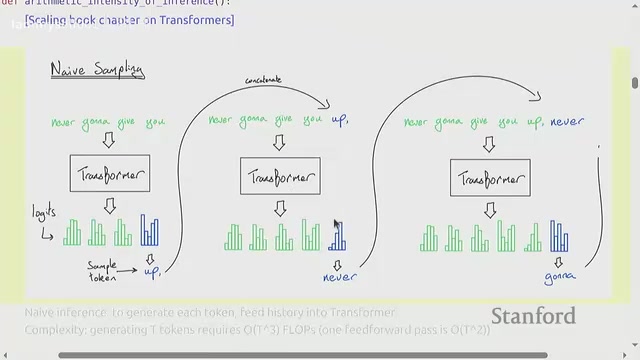
At the extreme — when B=1, equivalent to a matrix-vector product — arithmetic intensity is approximately 1, which is very bad. You are reading the entire D×F matrix from memory while performing roughly the same number of FLOPs, and memory reads are extremely slow. This is precisely what happens during token-by-token generation: arithmetic intensity is near 1, making generation inherently memory-limited.

Arithmetic intensity measures the ratio of computation to memory access, in units of FLOPs/Byte. GPU hardware has a "roofline" threshold: when arithmetic intensity exceeds it, the bottleneck is the compute units (compute-bound) and the GPU's matrix cores are fully utilized; below it, the bottleneck is memory bandwidth (memory-bound), and most time is wasted waiting for data to transfer from VRAM to compute units. The H100's peak arithmetic intensity is roughly 295 FLOPs/Byte, meaning for every byte read from VRAM, 295 floating-point operations are needed to keep the GPU busy. Large matrix multiplications during batch training easily clear this bar. But during inference, batch sizes are often small or even 1, meaning the vast majority of inference time is spent waiting on memory rather than computing — the GPU's peak compute is severely underutilized.

KV Cache: The Cure That Becomes a New Bottleneck

The most naïve generation approach re-feeds the entire sequence into the Transformer for every new token, resulting in O(T²) complexity and massive redundant computation. For autoregressive causal Transformers, the encoding of the prefix can be reused — and this is the idea behind the KV cache.

Inference is thus split into two phases: prefill encodes the prompt in parallel and computes the KV cache — this step is parallelizable, fast, and compute-bound, so it's relatively comfortable; generation then produces tokens one at a time sequentially, which is the root of the efficiency problem.

By computing arithmetic intensity separately for MLP and attention layers, the lecturer arrives at a key insight. For MLP layers, arithmetic intensity is B×T; during generation T=1, so you need a sufficiently large batch size (i.e., concurrent requests) to improve efficiency. For attention layers, arithmetic intensity is S×T/(S+T), which during generation is approximately 1 — and completely independent of batch size. The reason: in MLP layers, every sequence hits the same weights, so they can be batched together and amortized; in attention layers, each sequence has its own unique KV cache — "every sequence is a special snowflake" — so batching provides no savings.

The Latency-Throughput Tradeoff

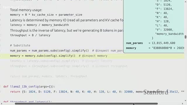
Using Llama 2 13B on an H100 as a back-of-the-envelope example: at batch size 1, latency is around 8ms per token and throughput is about 124 tokens/sec. As batch size grows to 16 and then 64, latency increases but throughput rises significantly. At 256, throughput gains start to plateau with diminishing returns, and the configuration requires roughly 240GB of memory — far beyond what a single H100 can hold.

This reveals the core tradeoff: small batches give better latency, large batches give better throughput, but the maximum batch size is capped by memory. Compared to the complex parallelism strategies used in training, inference has an extremely simple parallelism option — just launch m copies of the model, with no communication overhead, no latency increase, and m times the throughput. Model and KV cache sharding is only necessary when the model is too large to fit on a single device.

Architectural Tricks for Shrinking the KV Cache

Since inference is memory-limited and the KV cache is the bottleneck, reducing cache size is key to acceleration — as long as it doesn't excessively harm accuracy. The lecture systematically covers several architecture-level methods for reducing KV cache size:

Grouped Query Attention (GQA): A middle ground between multi-head attention and multi-query attention, GQA reduces the number of key-value heads so that multiple query heads share one set of KVs. Experiments on Llama 2 13B with a 1:5 ratio show lower memory usage, significantly higher throughput, and nearly unchanged accuracy. Llama 3 broadly adopted GQA precisely due to inference cost considerations.

Multi-head Latent Attention (MLA): From DeepSeek^Ad V2, this approach doesn't change the number of KV heads but instead projects them into a low-dimensional space — aggressively compressing from 16,000 dimensions down to 512. The only complication is incompatibility with RoPE, requiring a small number of extra dimensions.

Cross-Layer Attention (CLA): While GQA shares across heads, CLA shares the same key-value projection across layers, improving the Pareto frontier between accuracy and cache size.

Local Attention: Attends only to the past K tokens, keeping KV cache size constant rather than growing with sequence length. Pure local attention degrades long-range dependency modeling, so it is typically interleaved with global attention — Character AI uses a hybrid scheme with 1 global attention layer per 6 local ones, combined with cache sharing.

Beyond Transformers: State Space Models and Diffusion Models

More radical approaches step outside the Transformer framework entirely. State Space Models (SSMs) originate from signal processing and control theory, initially conceived to address the quadratic cost of long-context modeling. Early work like S4 admits both RNN and convolution interpretations. However, SSMs struggled with language modeling — the sticking point being "associative recall" tasks that require precisely locating a key-value pair and retrieving the answer. Successive works — Hyena, H3, Mamba — progressively improved on this; Mamba has been scaled by AI21 to a 52B MoE, though it still requires one Transformer layer every 8 layers.

Linear attention has recently seen a renaissance. By applying a Taylor expansion to the attention kernel, the computation is rewritten as a dot product of nonlinear mappings, making it linear in sequence length rather than quadratic — behaving like an RNN. Minimax has used this approach to train a 456B MoE, replacing most layers with more efficient linear or local attention while retaining full attention only occasionally.

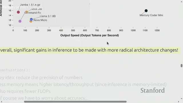
Diffusion models break free from autoregressive constraints entirely, generating all tokens in parallel and refining them iteratively. Models from Inception Labs achieve tokens/sec on coding tasks that far exceed any Transformer or hybrid architecture like Jamba. The lecturer argues that even if diffusion models incur some accuracy loss, their enormous speed advantage leaves plenty of headroom to compensate by spending more compute.

The core idea behind State Space Models (SSMs) comes from classical linear dynamical systems: a hidden state vector h compresses all historical information, updated each step from the current input and then mapped to the output. This means inference requires O(1) memory and compute (only the current state, no KV cache), while Transformer KV caches grow linearly with sequence length. During training, SSMs can be equivalently rewritten in convolutional form, enabling parallel processing of the full sequence for efficiency. Mamba's key innovation is the "selective" mechanism (Selective State Space), which makes state transition matrices dynamically input-dependent, overcoming early SSMs' weakness at content retrieval. The tradeoff is that precise multi-hop reasoning or very long-range information retrieval still falls short of full attention — which is why existing hybrid architectures retain a small number of Transformer layers.

Quantization, Pruning, and Speculative Decoding

Beyond architectural changes, there are several general-purpose techniques. Quantization reduces numerical precision: FP32 for training, BF16 as the inference default, with further options of FP8, INT8, and even INT4. The challenge is that outliers in large networks can break low-precision performance. LLM.int8 handles large outliers separately in 16-bit while using INT8 for everything else; Activation-Aware Weight Quantization (AWQ) uses activation values to determine which weights deserve preserved precision.

Model pruning uses a small calibration set to identify important layers, heads, or hidden dimensions, removes the unimportant ones, and then applies distillation from the original model to recover the pruned model's performance. Some work has pruned a 15B model to 8B with nearly no accuracy loss; pruning to 4B shows some degradation.

Speculative Decoding is the most elegant solution — it lets you have your cake and eat it too. It exploits an asymmetry: prefill (verification) is faster than generation. A cheap draft model speculatively generates K tokens ahead, and the target model then verifies them in parallel, accepting each token with probability Q/P (a rejection-sampling / Metropolis-Hastings approach). This guarantees the resulting samples are statistically identical to running the target model alone, and in practice delivers roughly a 2× speedup. A typical configuration pairs an 8B target model with a 1B draft model. Improvements like Medusa and Eagle allow the draft model to sample in parallel or reuse high-level features from the target model.

The correctness guarantee of speculative decoding deserves special mention. Draft tokens are not accepted directly — they pass through a strict accept-reject step: for the i-th draft token x, it is accepted with probability min(1, P_target(x)/P_draft(x)); otherwise a corrected sample is drawn from a modified distribution. This mechanism is mathematically equivalent to the Metropolis-Hastings algorithm, guaranteeing that the output token sequence has exactly the same statistical distribution as running the target model alone. This is unlike knowledge distillation or quantization, both of which alter the output distribution — speculative decoding is lossless acceleration. The speedup depends on the draft model's "hit rate": if the draft and target models are similar enough (e.g., small and large versions of the same family), most tokens are accepted and the average accepted length per verification batch approaches K, nearing the theoretical K× speedup. If the two models differ substantially, frequent rejections introduce overhead.

System-Level Serving Optimizations

In real serving scenarios, requests arrive at different times, finish at different times, may share prefixes, and vary greatly in length — the workload is highly heterogeneous. Continuous batching allows new requests to be inserted at any time without waiting for an entire batch to finish; selective batching handles attention separately while flattening variable-length tensors together for MLP computation.

PageAttention (the technology behind vLLM) borrows from OS virtual memory: it divides the KV cache into contiguous blocks allocated on demand, solving memory fragmentation; for shared prefixes it uses copy-on-write with reference counting to save memory.

Continuous batching addresses the inefficiency of traditional static batching. Static batching requires all requests in a batch to start and finish together — short requests must wait for the longest one before resources are freed, leading to poor GPU utilization. Continuous batching treats the inference server as a pipeline: after each iteration, it checks whether any requests have finished generating, removes them from the batch, and immediately fills the slot with a new request from the queue, keeping the GPU fully occupied at all times. PageAttention slices the KV cache into fixed-size "pages" analogous to OS physical memory pages. It eliminates the need to pre-allocate contiguous maximum-length memory for each request, removing internal fragmentation. It also allows multiple requests sharing the same prefix (e.g., a system prompt) to map to the same physical memory block via a page table, significantly reducing VRAM usage — this is the core reason vLLM achieves such substantial throughput improvements.

Conclusion

The world of inference is far broader than "deploying a chatbot." It is memory-limited and dynamically varied, presenting a range of challenges that simply do not exist in training. Real performance breakthroughs rarely come from system optimization alone — they come from fundamental architectural changes. The question you are always really asking is not "how do I run this specific model" but "how do I deliver the best accuracy within a given resource budget." Whether you are shrinking the KV cache, rethinking the Transformer, or moving toward SSMs and diffusion models, the underlying goal is always the same: routing around the fundamental obstacles of inference.