Building HNSW by Hand in TypeScript: Measuring the efSearch–Recall Tradeoff
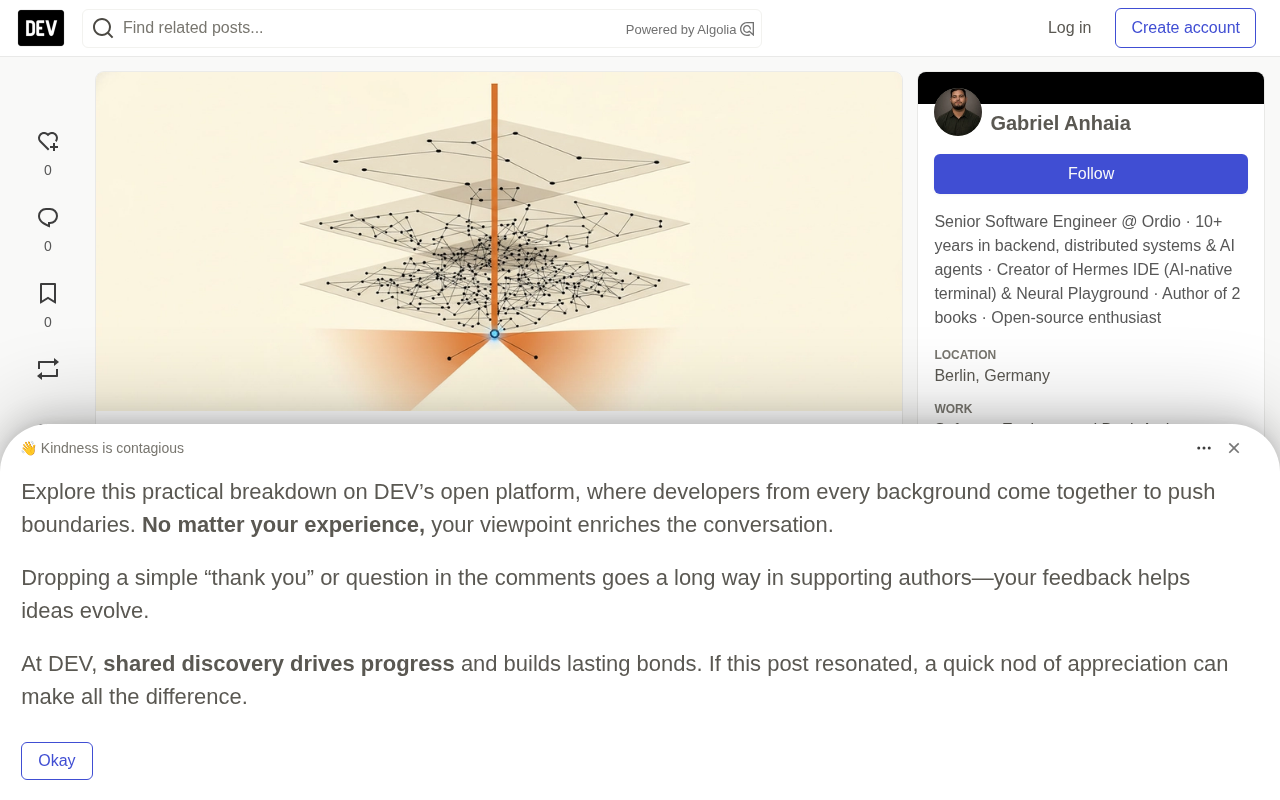
A hand-written mini HNSW in TypeScript measures how efSearch determines RAG retrieval recall.
Starting from pgvector's default hnsw.ef_search=40, the article notes that most Postgres RAG apps have retrieval quality decided by this rarely-changed parameter. The author builds a deterministic mini HNSW in one TypeScript file, indexes 50,000 random vectors, and compares recall@10 against brute force at efSearch 10, 40, 100, and 200, explaining layering, greedy descent, beam search, and why the neighborhood heuristic is key to navigability. It also covers interpreting results: random vectors are the worst case; brute force is the exact baseline; pgvector's filter-after-index shrinks a small beam; production tuning via SET LOCAL or enable_indexscan=off and Qdrant's exact flag enables recall monitoring.
pgvector's README sums up the cost of approximate indexing in a single sentence: adding an index means "trading recall for speed." The default hnsw.ef_search is 40—so if your RAG application runs on Postgres and nobody on the team has ever changed this value, then this 40 is what decides which chunks your model gets to read.
Rather than reading about it in the docs, it's better to build the index yourself and watch it happen. The path below writes a mini HNSW in TypeScript, indexes 50,000 random vectors in Node, then compares recall@10 against brute-force search at efSearch values of 10, 40, 100, and 200. The script is deterministic (the same data produces the same results on every run) and short enough to read in one sitting.
Three Core Concepts: Layers, Greedy Descent, Beam Search
HNSW comes from Malkov and Yashunin's 2016 paper on hierarchical navigable small world graphs. Set aside the proofs and three ideas remain.
Layering. Every vector lives on layer 0; a small random fraction also exists on layer 1, fewer still on layer 2, and so on. The paper defines an element's top layer as floor(-ln(uniform) * mL), recommending mL = 1/ln(M), where M is the number of links per node. The result resembles a skip list: sparse upper layers handle long jumps, dense lower layers ensure precision.
Greedy descent. A query starts from an entry point on the top layer, walks toward closer neighbors until none are closer, then drops down a layer and repeats. Upper-layer search uses ef = 1: keep a single candidate, pure greed.
Beam search at the bottom. The bottom layer maintains a candidate list of size ef, repeatedly expanding the nearest unexpanded node until the nearest unexpanded candidate is farther than the worst node in the list. This ef is efSearch. The wider the beam, the more of the graph you explore, the more true neighbors you find, and the more distance computations you pay.
HNSW's full name and positioning. HNSW stands for Hierarchical Navigable Small World—the layered version of the navigable small world graph. Its predecessor NSW (navigable small world graph) was proposed by the same authors, with the core observation that once high-dimensional vectors are built into a graph, any two points can connect in very few hops, and a search can rapidly approach the target by greedily following edges that head "closer to the goal." But NSW easily falls into local optima on low-dimensional or strongly clustered data. HNSW solves this by stacking multiple sparse layers: upper layers are sparse, have few edges, and cover long distances for coarse localization; lower layers are dense, have many edges, and offer high precision for fine search. This "multi-resolution" idea belongs to the same design family as skip lists, B-trees, and image pyramids, and it's why HNSW dominates vector databases. Understanding this is what lets you see why efSearch only affects the width of the bottom-layer beam search and not the greedy path above.
Minimal Implementation: From Vector Generation to Insertion and Search
All code goes in a single file hnsw.ts, appended in order. Node since v22.18.0 and v23.6.0 strips types and runs .ts files directly, with no build step. The code deliberately avoids enums and parameter properties, since type stripping doesn't support those two syntaxes.
A few key tradeoffs: a seeded random number generator via mulberry32 ensures every machine produces the same 50,000 vectors, making runs comparable; distance uses squared L2, which on unit vectors ranks identically to cosine similarity (|a - b|² = 2 - 2·cos(a, b)); an ordered array replaces the paper's two priority queues—slower at beam widths of a few hundred but readable and correct, and readability matters more here.
searchLayer corresponds to Algorithm 2 in the paper, selectNeighbors to the neighborhood heuristic (Algorithm 4, minus the optional extensions), and insert and search to Algorithms 1 and 5. 1 - this.rand() keeps the logarithm away from ln(0), since the generator may return 0 but never 1. search clamps the beam width to at least k, matching hnswlib's parameter note: ef "can't be set smaller than the number of nearest neighbors k."
The neighborhood heuristic is what keeps the graph navigable. Connecting directly to the nearest M points sounds reasonable, but on clustered data the links get trapped inside each cluster and search stalls at cluster boundaries. Figure 7 in the paper demonstrates this: the simple rule plateaus at low recall on clustered data, while the heuristic doesn't.
The relationship between hnswlib and pgvector. The article repeatedly references hnswlib's parameter documentation because pgvector's HNSW index implementation draws on hnswlib's algorithms and defaults, though it doesn't embed the library directly—pgvector rewrote it in C and adapted it to Postgres's storage layer. hnswlib is a standalone C++ header-only library maintained by Malkov and colleagues, and it's the algorithmic prototype for many vector databases (including some versions of Qdrant and historical Milvus implementations). That's why hnswlib's description of ef—higher means more accurate but slower, and it can't be smaller than k—carries over almost directly to understanding pgvector's hnsw.ef_search. The difference is that pgvector exposes index parameters as GUC variables and index options (WITH (m = 16, ef_construction = 64)), whereas hnswlib passes them as function arguments at build and query time.
Benchmark: recall@10 vs. Brute Force
The benchmark builds the index with M = 16 and efConstruction = 64 (pgvector's defaults), computes exact answers via brute force, then sweeps efSearch.
With over 50,000 insertions, each a pure-JavaScript beam search with no SIMD, building the index is the slow part. To see a first result faster, drop N to 10,000.
recall@10 is averaged over 500 queries: how many of HNSW's 10 results fall within the true nearest 10. Timing wraps only the search call, so recall bookkeeping doesn't leak into per-query latency.
No results table is printed here, because the only numbers worth trusting are the ones from your own machine. Documentation can only predict direction: pgvector says higher ef_search gives "better recall" at the cost of speed, and hnswlib says "the higher ef, the more accurate but slower the search." Your run tells you the magnitude, and whether going from 40 to 100 buys more than going from 100 to 200.
How to Read Your Numbers
Random vectors are the hardest case. Uniform random data has no clusters, and its intrinsic dimensionality approaches its nominal dimensionality. Elliott and Clark's paper ties HNSW recall to data intrinsic dimensionality and insertion order, while Marqo's article on HNSW recall notes that clustered data "tends to yield higher recall than uniformly distributed data." Real text embeddings have structure, so treat recall on random data as a pessimistic floor. Try DIM = 16 and DIM = 256 (the latter with a smaller N, since each distance computation costs four times as much) to see how differently the same efSearch performs.
The brute-force line is your baseline. At 50,000 vectors an exact scan is cheap; it's what pgvector does without an index, with perfect recall. HNSW only pays off as N grows: brute force scales linearly with the corpus, while graph search is roughly logarithmic per the paper.
Filtering makes a small beam even smaller. pgvector applies WHERE filters only after the index scan. Its README states the consequence directly: "If a condition matches 10% of rows, with HNSW and the default hnsw.ef_search of 40, on average only 4 rows will match." That is, a top-10 query returns only 4 rows. Since 0.8.0, pgvector offers iterative index scans that keep scanning until enough rows pass the filter.
Turning this knob in production. In Postgres it's just a setting, scoped to a transaction: BEGIN; SET LOCAL hnsw.ef_search = 100; SELECT id FROM chunks ORDER BY embedding <=> $1 LIMIT 10; COMMIT;. In Qdrant you pass "params": { "hnsw_ef": 128 } per search; its indexing docs say ef defaults to the value of ef_construct, which is 100 out of the box.
Both stores also let you bypass the index for exact answers: pgvector with SET LOCAL enable_indexscan = off inside a transaction (the README recommends this for monitoring recall), and Qdrant with "exact": true. This exact path is how you build your own recall test on real data: take a few hundred real queries, compute the exact top-10 once, then compare what your production settings return.
Iterative index scan. This is the mechanism pgvector 0.8.0 introduced to mitigate the "index scan first, filter later" shortfall. In default mode, HNSW pulls a fixed number of candidates based on ef_search and stops, then applies WHERE to that batch—returning fewer than k rows if too few match. With iterative scanning enabled (SET hnsw.iterative_scan = relaxed_order or strict_order), pgvector keeps expanding the scan when candidates run out, until it collects enough rows to satisfy the LIMIT or hits the hnsw.max_scan_tuples cap. strict_order guarantees strictly distance-ordered results but is slightly slower; relaxed_order permits approximate ordering with higher throughput. The cost is that when filter selectivity is extremely low, a single query scans a large number of graph nodes and latency rises—so it suits RAG scenarios that "need top-k after filtering," but not high-concurrency queries with extremely sparse filter conditions.
What This Toy Implementation Leaves Out
A real implementation still needs what this single file skips: deletion and updates, concurrent insertion, on-disk page storage, quantized vectors, SIMD distance kernels. The paper's neighborhood heuristic also has two optional switches (extend candidates, keep pruned connections), neither enabled here.
To see why the heuristic exists, swap the generator for clustered vectors, replace selectNeighbors with a plain slice of the nearest M candidates, and compare recall at the same efSearch.
One-line Summary
A hand-written mini HNSW in TypeScript measures how efSearch determines RAG retrieval recall.
Paragraph Summary
Starting from the fact that pgvector's default hnsw.ef_search is 40, the article notes that most Postgres RAG applications have their retrieval quality decided by a parameter almost nobody changes. The author implements a deterministic mini HNSW in a single TypeScript file, indexes 50,000 random vectors, uses brute force as the baseline, compares recall@10 at efSearch values of 10, 40, 100, and 200, and explains the three core mechanisms—layering, greedy descent, beam search—along with why the neighborhood heuristic is key to graph navigability. The article further explains how to interpret the measured numbers: uniform random vectors are the worst case while real embeddings have structure and thus higher recall; brute force is the exact baseline; pgvector's index-then-filter design makes a small beam even smaller; production can tune per transaction with SET LOCAL, or build recall monitoring via enable_indexscan=off and Qdrant's exact parameter.
Related articles

Cursor AI Programming in Practice: Build a Student Management System from Scratch in 30 Minutes
A Bilibili creator demonstrates Cursor AI programming: generating a student management system in 30 minutes with natural language. Details on Agent mode, Claude selection, prompt techniques, and thresholds.

Top 20 AI Coding Tools Ranking: From Rock-Solid to Lackluster, a Scored Matrix
Bilibili creator releases top 20 AI coding tools ranking, tiered T0–T4 from rock-solid to lackluster, with Claude Code and Codex tied at T0. This article details the scoring dimensions (capability, reliability, robustness, durability, cost, domestic availability) and tool performances to help developers choose the right AI coding assistant.

Vibe Coding Systematic Tutorial: Master AI-Assisted Programming from Zero
A three-month Vibe Coding tutorial from a Bilibili creator covering Codex, ClaudeCode, and Cursor, from core logic to commercial project practice for beginners.