Can Stiff ODE Solvers Accelerate Neural Network Training?

A Forgotten Idea for Faster Training

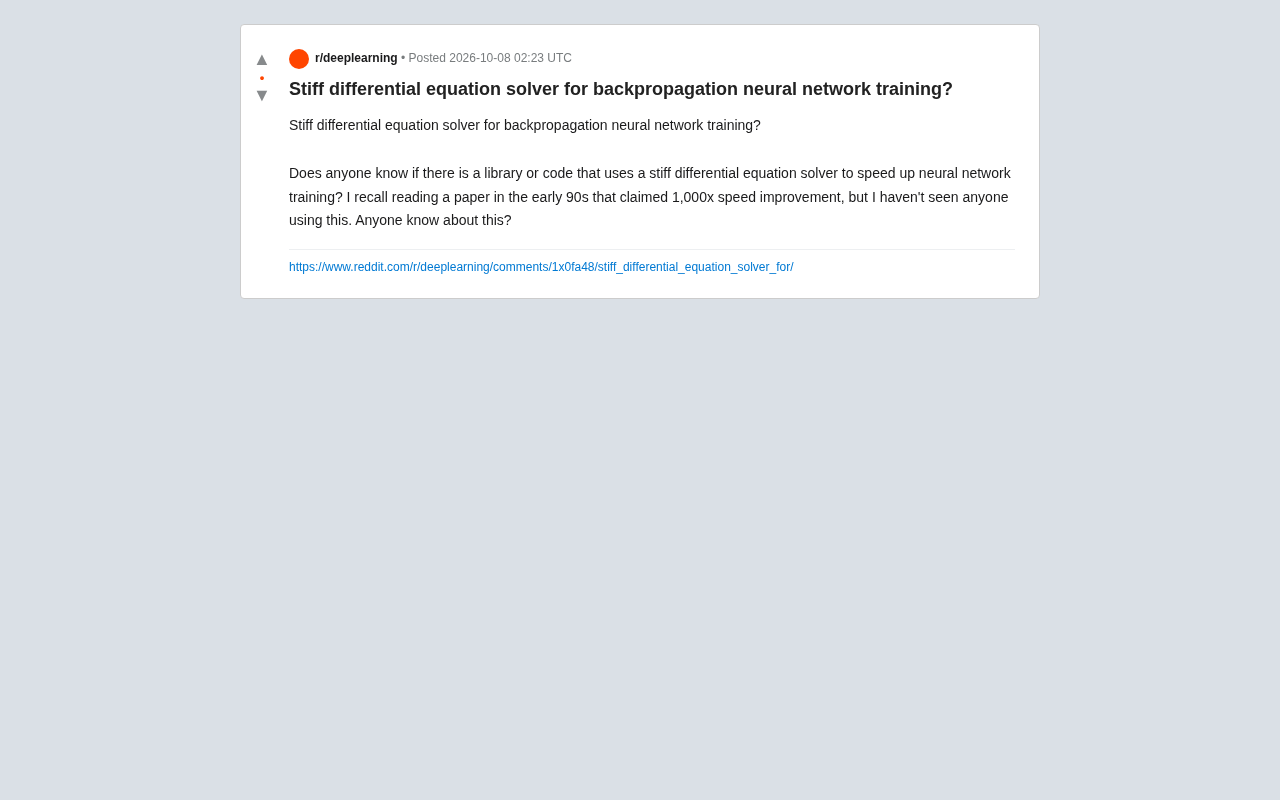
In a machine learning discussion on Reddit, a user raised a question with surprising historical depth: are there any libraries or code that use stiff ODE solvers to accelerate neural network backpropagation training? The poster recalled reading a paper in the early 1990s claiming this approach could achieve up to 1000× speedup in training — yet they never saw anyone actually use it afterward.

The question may seem obscure, but it touches on a fundamental perspective on neural network training: viewing the training process as the evolution of a continuous dynamical system, rather than a sequence of discrete gradient descent steps. It's worth unpacking the underlying principles and where things stand today.

Why Training Can Be Viewed as a Differential Equation

Standard backpropagation is essentially a discrete iteration of gradient descent: parameters are updated step by step in the direction of the negative gradient of the loss function. If we treat the learning rate as an infinitesimally small time step, this discrete process converges to a continuous gradient flow ODE:

dθ/dt = −∇L(θ)

From this perspective, training a neural network is equivalent to numerically integrating the ODE above. Ordinary gradient descent corresponds to solving it with the simplest explicit Euler method — and numerical analysis has long told us that Euler's method is extremely inefficient for stiff equations, requiring very small step sizes just to remain stable.

What Is Stiffness?

Stiffness refers to a system where components with vastly different rates of change coexist: some directions converge extremely fast, others extremely slowly. For a loss surface, this corresponds to a Hessian matrix with a large condition number — widely varying curvature across different parameter directions. In this case, the step size for explicit methods is constrained by the "fastest" component, causing the overall convergence to be painfully slow. Implicit stiff solvers (such as BDF and implicit Euler) can maintain stability with large step sizes — and that is the theoretical basis for the claimed "1000× speedup."

A classic example of a stiff equation is chemical reaction kinetics: in a reaction network, some intermediate species decay within microseconds while others take hours to reach equilibrium, all coexisting in the same system. For neural networks, the ratio of the largest to smallest eigenvalue of the Hessian (i.e., the condition number) measures the degree of stiffness. Research shows that the Hessian condition number of deep networks can easily reach 10⁴ to 10⁶, meaning the explicit Euler step size must shrink to the level demanded by the fastest component, while the overall trajectory may require tens of thousands of steps for the slowest components to converge. Implicit stiff solvers such as BDF (Backward Differentiation Formula) and Radau handle fast components with "unconditional stability" by implicitly solving a system of equations at each step, allowing step sizes to be dictated by accuracy requirements rather than stability constraints — this is the mathematical root of why the theoretical speedup ratio can be so large.

What That 1990s Paper Likely Referred To

The poster didn't provide an exact citation, but based on the timeframe and description, this work likely belongs to an early wave of research on optimizing neural network training through the lens of ODEs. Researchers noticed that one root cause of slow backpropagation convergence was the stiffness of the loss surface, and proposed using implicit integration or variable-step stiff solvers to take larger "time steps" across flat regions.

In theory, if training dynamics are highly stiff, speedups of several orders of magnitude from implicit methods are not far-fetched. But extreme numbers like "1000×" typically appear on specific small-scale constructed problems and are difficult to generalize directly to large, real-world networks. This is likely one reason the approach was never widely adopted.

Why It Never Became Popular

From an engineering standpoint, there are several key barriers that prevented stiff solvers from becoming mainstream training methods:

• Implicit solvers require solving linear systems at each step, relying on second-order information like the Hessian or its approximation — the computational and memory cost is enormous at scales of millions or billions of parameters.
• Modern deep learning loss surfaces are non-convex, high-dimensional, and stochastic — the noise introduced by mini-batches undermines the value of "precisely integrating an ODE," since we don't need to faithfully trace a deterministic trajectory.
• Adaptive optimizers (Adam, RMSProp, etc.) already partially address stiffness in a cheap way, using per-coordinate adaptive step sizes to approximate the same effect — and are far simpler to implement.

In other words, the idea wasn't disproven — it was bypassed by more practical and scalable alternatives.

K-FAC (Kronecker-Factored Approximate Curvature) and Shampoo are two representative modern second-order/higher-order optimizers that serve as practical approximations to the implicit stiff solver approach. K-FAC exploits the Kronecker decomposition structure of the Fisher information matrix to compress the otherwise O(n²) curvature matrix into the product of two smaller matrices, making the preconditioned step computationally feasible. Shampoo maintains second-order statistics separately along each dimension of every parameter tensor, also avoiding full Hessian computation. In large-batch training scenarios, these methods often reach the same loss with fewer iterations for the same computational budget — mathematically consistent with the original intent of "using large steps to traverse stiff directions." Their existence also explains why dedicated stiff ODE solvers have lacked traction in the optimization community: their core benefit has been absorbed in a more engineering-friendly form.

Modern Echoes of This Idea

It's worth noting that research connecting neural networks with differential equations has seen a resurgence in recent years. Neural ODEs model the forward pass of a network itself as a continuous dynamical system, integrating it with mature ODE solvers — including stiff solvers. Related frameworks like torchdiffeq and diffrax do include built-in stiff solver options, though their goal is modeling continuous dynamics rather than directly accelerating traditional backpropagation.

From an optimization perspective, second-order methods (such as K-FAC and Shampoo) and various preconditioning techniques are fundamentally fighting the "stiffness" of the loss surface — a direct continuation of the motivation behind that 1990s paper. In a sense, the idea the poster remembered lives on today, just in different forms.

Neural ODE (Chen et al., NeurIPS 2018) is the most influential modern embodiment of this idea. Its core insight is to take the limit of layer-by-layer transformations in a residual network into a continuous vector field dh/dt = f(h,t,θ), with network outputs obtained by integrating with an ODE solver. Gradients are computed in reverse via the adjoint method, eliminating the need to store intermediate activations and reducing memory complexity from O(depth) to O(1). However, when the vector field itself is stiff (e.g., when modeling physical or biochemical systems), one must switch to a stiff solver — such as Kvaerno5 in diffrax or dopri5 with stiffness detection in torchdiffeq — otherwise the solver gets trapped in an explosion of tiny steps and function evaluations. This is technically symmetric to the 1990s problem, except the stiffness now comes from the dynamics being modeled, rather than the optimization trajectory itself.

Practical Suggestions for the Original Poster

If you want to experiment with this idea, here are some starting points:

• Explore diffrax and torchdiffeq — they provide ready-to-use interfaces for stiff and implicit solvers.
• On small-scale problems, model training as a gradient flow ODE and compare the convergence step counts of explicit Euler (i.e., standard SGD) vs. implicit methods.
• To track down that legendary paper, try searching Google Scholar for terms like "stiff ODE neural network training" or "continuous backpropagation" — many 1990s papers have since been digitized.

This question is a reminder that many "new" ideas in machine learning have roots stretching back decades into numerical analysis and dynamical systems research. Revisiting these forgotten corners can sometimes yield unexpected inspiration.