Do You Need to Master the Math Behind Every Solver to Learn Machine Learning? A Layered Learning Strategy Guide

A Learner's Real Dilemma

Many machine learning beginners hit the same wall: just when you think you've thoroughly understood the math behind an algorithm, you open up a library and discover a pile of terms you've never seen before.

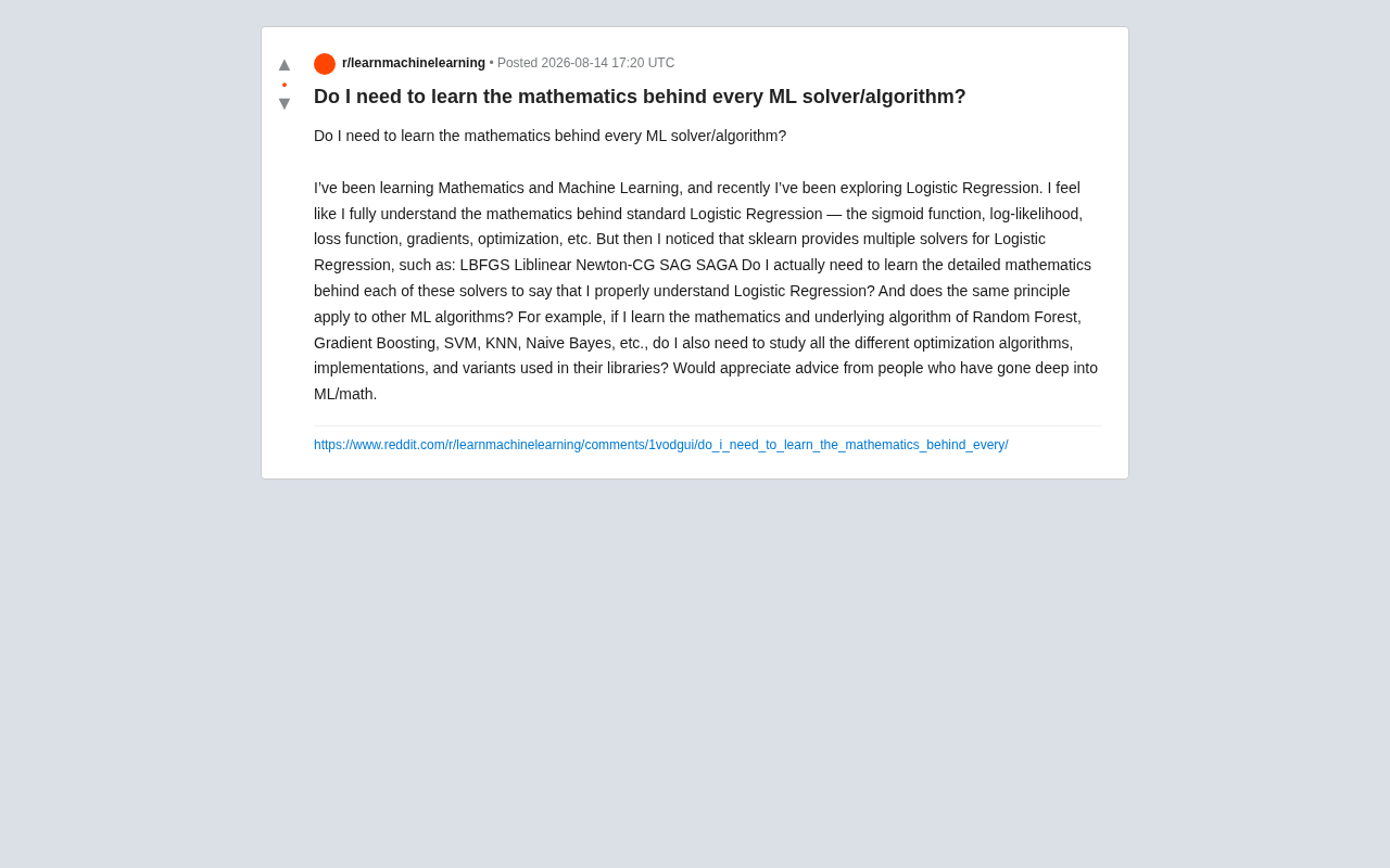
A Reddit user recently shared exactly this experience. They said they had fully mastered the math behind Logistic Regression — including the sigmoid function, log-likelihood, loss function, gradient, and optimization process. But when they opened scikit-learn, they found that logistic regression alone offers multiple solvers:

LBFGS
Liblinear
Newton-CG
SAG
SAGA

So they asked the question that nearly every ML learner eventually asks: Do I need to learn all the detailed math behind these solvers to truly understand logistic regression? And does this apply to Random Forest, Gradient Boosting, SVM, KNN, Naive Bayes, and every other algorithm?

reddit source

The question seems simple, but it touches on a core trade-off in the machine learning learning path: how to balance depth versus breadth.

Models and Solvers Are Two Different Layers

To answer this question, you first need to distinguish between two layers — model definition and optimization/solving.

The Model Layer: The Core Math You Must Master

Take logistic regression as an example. The model's mathematical definition is fixed and fundamental: it assumes the log-odds are a linear combination of features, maps them to probability space via the sigmoid function, and uses cross-entropy (log-likelihood) as the objective function. This layer determines:

What kinds of relationships the model can fit
What the parameters mean
When underfitting or overfitting will occur
How to interpret coefficients and make predictions

The math at this layer is non-negotiable. If you don't understand why we use the sigmoid or why the loss function takes that particular form, you can't judge whether the model is appropriate for your problem or debug unexpected results.

It's worth understanding deeply that the choice of the sigmoid function is no accident — it's the canonical link function for the Bernoulli distribution within the exponential family framework, rooted in the theory of Generalized Linear Models (GLM) from statistics. The log-likelihood loss (i.e., cross-entropy loss) is equivalent to Maximum Likelihood Estimation (MLE), which under correct model specification has asymptotically optimal statistical properties, including consistency and asymptotic normality — meaning parameter estimates converge to the true values as sample size grows. More importantly, logistic regression's loss function is convex, which guarantees that any local optimum is also the global optimum — this is the fundamental mathematical reason why different solvers ultimately converge to the same result.

The Solver Layer: Essentially "How to Find the Optimal Solution"

Solvers like LBFGS, SAGA, and Newton-CG are fundamentally solving the same problem: given a loss function, what numerical method should we use to find the optimal set of parameters?

The key insight is that they all converge to solutions that are mathematically identical or nearly identical (especially true for convex problems like logistic regression). Their differences lie in engineering trade-offs:

Liblinear: Suited for small datasets, supports L1 regularization
LBFGS / Newton-CG: Leverage second-order information, converge fast, suited for medium-scale problems
SAG / SAGA: Stochastic gradient methods suited for large-scale data; SAGA also supports L1

These five solvers actually represent decades of technical evolution in the field of numerical optimization. Liblinear originated from the work of Chih-Jen Lin's team at National Taiwan University in 2008, designed specifically for linear classifiers. It uses coordinate descent to update parameters one at a time and is highly efficient on small-scale, high-dimensional data. LBFGS (Limited-memory Broyden-Fletcher-Goldfarb-Shanno) is a representative quasi-Newton method that stores gradient difference information from the most recent m steps to approximate the inverse Hessian matrix, achieving near-second-order convergence speed with only O(md) memory. Newton-CG uses the conjugate gradient method to iteratively solve Newton's equation, avoiding explicit construction of the full Hessian matrix. SAG and SAGA belong to the variance reduction class of stochastic optimization methods, maintaining a history of per-sample gradients to achieve linear convergence rates while keeping per-step computation at O(1) — a theoretical breakthrough that ordinary SGD cannot match.

In other words, choosing a solver is more like choosing "which path to take up the mountain" rather than "which mountain to climb."

The Optimization Knowledge You Actually Need

Synthesizing the prevailing view among experienced practitioners in the community, the answer is layered: You need to understand the 'core idea' and 'use cases' of each optimization method, but you don't need to hand-derive the complete mathematical proof for every solver.

Build Transferable Optimization Intuition

Rather than grinding through sklearn's five solvers one by one, build a transferable optimization knowledge framework:

The gradient descent family: The differences and trade-offs between batch, stochastic, and mini-batch
First-order vs. second-order methods: Why Newton's method converges fast but is computationally expensive, and why quasi-Newton methods (like LBFGS) are a compromise
The impact of regularization: Why certain solvers only support specific regularization terms
The impact of data scale: How sample size and feature dimensionality affect solver selection

Regarding the distinction between first-order and second-order methods, it's worth building clearer intuition. First-order methods use only gradient information — essentially knowing only the "slope" at the current position and moving in the steepest direction. Second-order methods additionally leverage the "curvature" information encoded in the Hessian matrix — they know not just which direction to go, but how the terrain curves, allowing them to adaptively adjust step size. When the loss surface has wildly different scales across directions (high condition number), first-order methods oscillate back and forth in narrow "valleys," while second-order methods can cut straight across. However, full Newton's method requires O(d³) computational complexity to invert the Hessian matrix, which is unacceptable for high-dimensional problems. LBFGS is the classic solution that strikes a balance between the two.

Regarding regularization and solver compatibility, the technical reasons are also worth understanding. L2 regularization adds a sum-of-squared-parameters penalty to the loss function, and the objective function remains smooth and differentiable — all gradient-based methods can handle it directly. But L1 regularization adds a sum of absolute values, making the objective function non-differentiable at zero (creating "kinks"), which prevents traditional gradient methods from being applied directly. This is why LBFGS and Newton-CG don't natively support L1. Liblinear naturally supports L1 through coordinate descent, since you can independently solve the one-dimensional sub-problem with absolute values for each coordinate. SAGA introduces a proximal operator trick, decomposing each update step into a gradient step and a proximal projection step, precisely handling L1's non-smoothness while maintaining the excellent convergence properties of variance reduction.

Once you've mastered these general principles, you can quickly understand the positioning of any new solver in any algorithm library just by reading the documentation, without having to learn from scratch.

Layered Learning Strategy: Allocate Effort by Priority

For other algorithms (Random Forest, GBDT, SVM, KNN, Naive Bayes), the same principle applies:

First priority: Understand the algorithm's core assumptions, objective function, and decision logic
Second priority: Understand the key engineering optimizations in mainstream implementations (e.g., XGBoost's histogram algorithm, SVM's SMO solver)
Optional deep dive: Only when you need to research, improve, or debug the underlying implementation should you study the full derivation of each variant

The engineering optimizations mentioned here are indeed worth a brief elaboration. XGBoost's histogram algorithm is a textbook example of engineering optimization — traditional exact greedy splitting requires sorting continuous features and traversing all possible split points, with time complexity of O(n·d). The histogram algorithm discretizes continuous feature values into a fixed number of bins (typically 256), reducing split-point search complexity to O(bins) while compressing memory usage from 32/64-bit floating-point numbers to 8-bit integer indices. This "lossy" approximation has virtually no impact on model accuracy in practice but delivers orders-of-magnitude speed improvements, and was later further developed by LightGBM. SVM's SMO algorithm (Sequential Minimal Optimization), proposed by John Platt in 1998, decomposes the SVM's n-variable quadratic programming problem into a series of minimal sub-problems — optimizing only two variables at a time (the smallest update unit allowed by the equality constraint). This sub-problem has an analytical solution, eliminating the need for a general QP solver and making SVM training feasible on medium-scale data.

Learning Depth Depends on Your Career Goals

Ultimately, "how deep should I go" doesn't have a universal answer — it depends on your role:

Applied Engineer / Data Scientist

Understanding model-layer math plus intuition about optimization methods and their use cases is sufficient. Your value lies in correct model selection, reasonable hyperparameter tuning, and accurate interpretation of results — not in reinventing solvers. When a solver throws a warning (like "did not converge"), being able to judge whether to switch solvers, increase iterations, or scale your features is enough.

Researcher / Framework Developer

Then diving deep into the mathematical details of each optimization algorithm becomes necessary. Researchers need to understand why SAGA can simultaneously guarantee variance reduction and support sparse regularization before they can propose improvements.

Specifically, SAGA's variance reduction mechanism works like this: it maintains a "gradient table" storing the gradient computed for each sample the last time it was selected. At each iteration, a sample j is randomly chosen, the current gradient g_j^new is computed, and then (g_j^new - g_j^old + historical average of full gradients) is used as the gradient estimate. This estimate remains unbiased, but its variance naturally tends toward zero as parameters converge — because as parameters approach the optimum, the difference between new and old gradients becomes smaller and smaller. This allows SAGA to achieve a linear convergence rate with a fixed learning rate, combining the fast convergence of full gradient methods with the low per-step cost of stochastic methods. Understanding this level of design is what enables you to identify room for improvement — for example, its O(n·d) extra memory overhead can become a bottleneck in ultra-large-scale problems, and how to address this is an active research frontier.

A Pragmatic Learning Recommendation

Don't invalidate your understanding of an algorithm just because you haven't learned every detail. Perfectionism is often the enemy of efficiency in machine learning education. A healthier mindset is: first build a broad and solid core understanding, then go deeper on demand based on actual needs. When a particular solver actually becomes a bottleneck in your project, go back and study its paper carefully — at that point, your learning will be more targeted and much easier to absorb.

Conclusion

Back to the original question: you don't need to learn the complete math behind every ML solver. What you need is a deep understanding of the model itself and transferable intuition about optimization methods. Solvers are tools for achieving a goal — understanding their 'ideas' matters far more than memorizing their 'derivations.' Learning machine learning is a marathon. Allocate your cognitive budget wisely, and you'll go much further.