Generalized Gibbs Sampling: Composing Diffusion Models with Physical Context

Why a Single Large Model Can't Solve Joint System Sampling

Diffusion models have demonstrated remarkable capabilities in scientific discovery. Microsoft Research's BioEmu can generate protein conformational samples from given sequences, while MatterGen generates structures for inorganic materials. Given sufficient training data, these end-to-end models perform exceptionally well. But Wei Zhou, a PhD student in Aaron Dinner's group at the University of Chicago and co-advised by John Zhang at NYU, pointed out in an academic talk that real-world training data rarely meets this ideal.

The problem centers on three issues. First is combinatorial scarcity: data on monomeric proteins is abundant, but when you want to train a model for protein dimers or larger assemblies, data volume falls far behind the explosive growth of the combinatorial space. Second is circular dependency: for an end-to-end model to work perfectly, you essentially need data from the target distribution to train it — but if you already have data from the target distribution, why train a model to generate it? Third is the modularity problem: pretrained models are typically trained under standard conditions (pure water, room temperature, no binding partners), and once conditions change (adding ions or binding partners), these scenarios are almost entirely out-of-distribution, making generalization difficult.

All three problems point to the same conclusion: the bottleneck isn't building stronger end-to-end models, but rather how we use models. Real physical systems are too diverse — trying to cover everything with a single model is bound to fail.

The Compositional Approach: Assembling Models at Inference Time

Wei Zhou's proposed solution is called "composition." Take a system consisting of two polymer chains — one red, one black — plus surrounding solvent and ions. The full system state S can be decomposed into subsystems: the red polymer, the black polymer, and the solvent and ions.

Rather than training a model that handles everything, the idea is to leverage existing monomer models — which have ample data and are well-trained — along with force fields that physicists have developed to high accuracy for describing solvent and inter-component interactions, and combine them at inference time. This requires only pretrained models for each monomer, plus an energy term called the "physical context."

This context term describes what the models haven't seen: solvent, ions, and their interactions. It is essentially an energy term that can be computed directly, taking the familiar form of a Boltzmann distribution, with no need for a model to learn it. The pretrained models only know how each polymer behaves in isolation, and the context fills in what's missing for the joint system.

Reinterpreting the Denoising Process as Posterior Sampling

Making composition possible requires a reinterpretation of what diffusion models actually do. When training a diffusion model, you start from target data, apply a forward corruption kernel (typically linear Gaussian) to add noise, then train the model to learn the reverse denoising process. By Bayes' theorem, the denoising process is actually a "denoising posterior" — the posterior equals the prior times the likelihood, where the prior is the training data and the likelihood comes from the forward corruption process we defined.

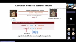
The key insight is: if instead of starting from pure noise you start from a specific diffusion timestep conditioned on a given noisy observation, the diffusion model is actually a posterior sampler drawing from a denoising posterior. Wei Zhou treats the denoiser as a black box — input a noisy observation and diffusion time, output a batch of samples — and builds the entire sampling theory on this foundation, without relying on any specific network architecture.

The forward process of diffusion models is typically defined as a linear Gaussian kernel: at each timestep $t$, the original data $x_0$ is progressively mixed with Gaussian noise until at $t=T$ the data is completely drowned in a standard normal distribution. The reverse process is trained by learning a denoising network (usually parameterized as a score function predicting noise) to gradually recover the data. From a Bayesian perspective, this reverse step can be interpreted as: conditioned on the noisy observation $x_t$, sampling from the posterior distribution $p(x_0 | x_t)$ of the original data $x_0$. This is the core property Wei Zhou exploits — the denoiser is naturally a conditional sampler, not merely a generator. The advantage of this perspective is that it turns "where to start the diffusion chain" into a controllable design parameter: starting from intermediate time $t^$ is equivalent to sampling from a posterior with $x_{t^}$ as the observation, allowing external physical constraints to be injected as "observations" without retraining the model.

The Generalized Gibbs Sampling Framework

Building on this understanding, the author constructs a family of joint distributions over diffusion time t. It consists of two parts: a context factor contributing the missing terms not modeled by the pretrained prior, and a product of all pretrained priors, connected by the forward kernel (linear Gaussian) used during model training.

This joint distribution is meaningful because it satisfies a "zero-time limit": as diffusion time approaches zero and the forward kernel degenerates to a delta function, integrating out the model variables leaves exactly the compositional target defined earlier. Furthermore, Proposition 1 proves that if the system is decomposable (total energy equals the sum of isolated subsystem energies plus environment energy and interactions), and each model is perfectly trained on its isolated component, with the context factor handling the remaining energy terms, then the joint distribution converges to the true physical distribution in the zero-time limit.

Sampling proceeds via a Gibbs approach, alternating between two steps. The first step fixes the full system state and updates the variables associated with each pretrained model — this is exactly denoising posterior sampling. The second step, called "context-aware aggregation," fixes the model variables and updates the full system state, with an effective energy comprising two parts: the full system energy term (governing environment and interactions), and a constraint term that pins part of the full system's degrees of freedom to the current model variables. These two steps alternate to form a Markov chain that eventually converges to the target distribution.

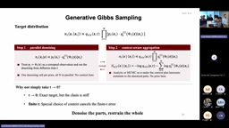
A subtle point: at zero time, the Markov chain cannot move at all (the denoiser outputs identically, and the constraint term becomes infinite), so a finite time must be chosen — which introduces error.

Gibbs sampling is a classic algorithm among Markov Chain Monte Carlo (MCMC) methods: when facing a multivariate joint distribution, it updates one variable (or a group of variables) at a time, fixing all others and sampling from the corresponding conditional distribution, iterating until convergence to the target joint distribution. Its strength is that when the joint distribution is hard to sample from directly, conditional distributions often have simpler, tractable forms. The "generalized" aspect here manifests in two ways: first, the sampling space is augmented to include diffusion time $t$, allowing the denoising posterior to be used directly as a conditional sampling step; second, different subsystems can use heterogeneous models (neural network denoisers and analytic force fields), each responsible only for its own degrees of freedom, coupled at inference time via the context factor rather than sharing a single parameterized model. This design allows the framework to theoretically inherit the convergence guarantees of Gibbs sampling while practically bypassing the need for unified training data.

Unbiased Sampling Under Quadratic Interactions

Here a beautiful result emerges. If the interactions between components in the target physical system are quadratic, because the forward kernel is itself linear Gaussian, one can always find an appropriate context time schedule such that the marginal distribution over x is exactly unbiased at finite time — if and only if the chosen context schedule satisfies two specific conditions.

In other words, as long as the injected noise doesn't exceed a certain upper bound, one can find a context factor that makes sampling exact at finite time. However, to ensure the covariance matrix remains positive definite, an upper bound on diffusion time is required. Smaller times slow down mixing, so the authors use "replica exchange over diffusion time" to accelerate — constructing replicas at larger diffusion times and exchanging between them, speeding up mixing while keeping the minimum-time replica unbiased.

This stands in sharp contrast to existing approaches. Whether split-Gibbs sampling, guided diffusion, or score composition, all require all models to operate in the same shared space; generalized Gibbs sampling defines an augmented space where each model controls only part of the joint system's degrees of freedom, with the rest governed by the physical model, enabling heterogeneous modeling of the joint system. In standard split-Gibbs, covariance mismatch causes "covariance inflation" leading to bias, while this framework only requires correcting the covariance as per Proposition 2 to remain unbiased for any linear inverse problem at any time below the upper bound.

Replica Exchange (also known as Parallel Tempering) is a standard technique for overcoming slow MCMC mixing: multiple Markov chains running at different temperatures (or noise levels) simultaneously exchange states between adjacent replicas periodically using the Metropolis criterion. High-temperature (high-noise) replicas easily cross energy barriers to explore large regions of conformational space, while low-temperature (low-noise) replicas precisely characterize the fine details of the target distribution; through exchanges, the low-temperature replicas leverage the high-temperature replicas' mobility for accelerated mixing without disrupting the stationary distribution. In this framework, "diffusion time" plays the role of "temperature": larger diffusion times correspond to replicas with stronger noise and looser denoising constraints, which mix faster but whose marginal distributions are no longer exactly the target; the minimum-time replica satisfies the unbiasedness condition and accelerates its mixing by exchanging states with large-time replicas, significantly improving sampling efficiency while maintaining accuracy.

Three Application Domains: From Lattice Models to Quantum Statistics

The framework covers three scenarios with identical sampling procedures; the only difference is whether the interaction type allows exact sampling at finite time.

Linear inverse problems correspond to a single prior plus a linear Gaussian context. The authors validate on a Gaussian mixture model: the error of standard split-Gibbs increases with the ratio, while this algorithm eliminates the painful tradeoff between accuracy and mixing through covariance correction.

Multiple priors with quadratic interactions correspond to scalar field lattice models and quantum statistics. In an L×L lattice model, spin interactions are quadratic — only a one-dimensional model needs to be replicated L×L times at inference time with quadratic interactions injected, and the algorithm correctly captures phase transition behavior. The quantum statistics application is particularly elegant: the path integral representation expands a system with nuclear quantum effects into multiple classical replicas coupled by quadratic interactions between adjacent replicas. This falls exactly within the exact regime — only a single denoising model trained on the classical Boltzmann distribution is needed, then combined at inference time.

Since all quantum information comes from quadratic terms combined at inference time, the framework brings unexpected flexibility: changing the mass simulates isotope effects, and changing the number of replicas p achieves temperature transferability. In tests on bulk water, a model trained only on classical statistical water boxes at 300K, combined with 32 replicas, naturally gives rise to quantum statistical behavior. Replacing hydrogen with deuterium or tritium produces more ordered structures, in good agreement with path integral molecular dynamics (PIMD) reference data. In terms of performance, since context aggregation is analytic and requires no evaluation of full-system energies and forces, this achieves approximately a 32× speedup over traditional PIMD methods.

Multiple priors with non-quadratic interactions is the final category, which introduces approximation errors. The authors study the alanine dipeptide system: a model trained on vacuum data has no knowledge of sodium ions, and direct sampling yields overly long oxygen-oxygen distances; combining sodium ions at inference time via the algorithm almost correctly recovers the oxygen-oxygen peak. Collective behaviors like parallel/antiparallel conformations of dipeptide dimers are also automatically reproduced, though some bias remains due to non-quadratic interactions.

Path Integral Molecular Dynamics (PIMD) is the standard computational chemistry method for studying nuclear quantum effects (NQE). Its theoretical foundation is Feynman path integrals: in thermodynamic statistics, a quantum particle can be equivalently represented as a ring polymer of $p$ classical "beads" connected by harmonic potentials, with the average position of all beads corresponding to the quantum particle's expected position. Larger $p$ (more replicas) gives more accurate quantum statistical descriptions but with linearly growing computational cost. Hydrogen atoms have small mass, making their zero-point energy and quantum tunneling effects particularly significant, and NQE substantially influences the structure and dynamics of water, proton conduction, and related systems. Traditional PIMD requires evaluating force fields or neural network potentials for all $p$ replicas simultaneously, while in this framework the harmonic coupling between replicas is exactly quadratic and can be handled analytically, with the neural network only needing to evaluate the denoising distribution of a single classical replica, achieving a dramatic reduction in computational cost.

Value and Limitations

The core thesis of this work is: studying joint distributions does not require a single monolithic end-to-end model — instead, the joint system can be decomposed into isolated components and recombined at inference time. The generalized Gibbs sampling framework is exact under quadratic interactions and introduces approximation errors in non-quadratic cases.

The author candidly acknowledges several future challenges. Because the framework repeatedly invokes the diffusion model, it amplifies the model's inherent errors — a single generation pass may look fine, but repeated use exposes model deficiencies, requiring the development of high-fidelity priors. Additionally, the framework needs to be extended beyond quadratic interactions, error control for non-quadratic cases needs to be developed, and extension to large biomolecular complexes remains an open challenge.

Discussion at the talk also touched on the method's boundaries: Gibbs sampling is fundamentally a framework and cannot guarantee that the model has been trained over the regions required by the joint distribution. If a certain configuration only appears in the presence of solvent but is never observed when looking at the solvent and molecule separately, Gibbs sampling will fail. For non-quadratic interactions, the fact that deconvolution has no solution means only times close to zero can be used, reverting to the slow-mixing problem — which is precisely the practical tradeoff this method must navigate.