Google TimesFM 3.0 Hands-On: Is Zero-Shot Forecasting Good Enough?

From ARIMA to Foundation Models: A Paradigm Shift in Time Series Forecasting

Most enterprises still follow the traditional path for time series forecasting: train a separate model for every series you need to track, fit it with ARIMA or gradient-boosted trees, tune the hyperparameters, then move on to the next series and repeat the whole process. If you manage a thousand stores, you theoretically need to maintain a thousand independent models. Language, code, and images have long been reshaped by foundation models, yet forecasting teams are still operating like a "manual workshop."

The TimesFM series from Google Research aims to break this mold. It is a decoder-only Transformer trained entirely on time series data, and its biggest selling point is zero-shot forecasting—no training on your business data required; it delivers predictions directly. The latest TimesFM 3.0 was pretrained on over one trillion time points, including both real series and a large amount of synthetic data.

The core idea is not complicated. It slices your historical data into 32-timestep "patches," treats each patch as a token, and then predicts the next stretch of the chart the way a language model predicts the next word. In the video author's words, this is "autocomplete for charts." Unlike a language model, it outputs not a single line but a daily median forecast plus an uncertainty interval, so you see both the most likely scenario and the downside risk at the same time.

ARIMA (Autoregressive Integrated Moving Average) is the classic statistical method for time series forecasting, consisting of three parts: autoregressive (AR), differencing (I), and moving average (MA). The AR term uses values from several past periods to predict the current value, the MA term corrects the current forecast using forecast errors from several past periods, and differencing removes trends and seasonality to make the series stationary. ARIMA requires the series to satisfy the stationarity assumption, and the orders are usually determined via ACF/PACF plots or information criteria (such as AIC); its ability to handle nonlinear relationships and external covariates is limited. Gradient-boosted trees (such as XGBoost and LightGBM) instead fit residuals step by step by ensembling many weak decision trees, automatically capturing nonlinearities and interaction effects, and perform excellently when feature engineering is thorough. But the fundamental limitation shared by both is that each model is trained for a single series or task and cannot transfer knowledge across series, which is why enterprises must repeatedly build and tune models for tens of thousands of series. This is precisely the "manual workshop" mode that foundation models aim to replace with pretraining plus zero-shot generalization.

The Key Upgrade in 3.0: Putting Covariates Inside the Model

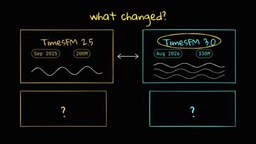
TimesFM 2.5 was released the previous year, and it works relatively simply: it forecasts one series at a time based only on historical values. If you want to account for known future events—an upcoming holiday or a planned promotion—you need to perform a separate regression fit outside the model, then have TimesFM forecast the residual portion that the regression did not explain. This pipeline works, but the tangled external steps add engineering complexity.

Version 3.0 moves the entire mechanism inside the model. You can feed in multiple related series and their historical values at once, and you can also pass future covariate inputs directly. Inside the Transformer, each token "looks ahead" at those upcoming input signals, so before forecasting a given week the model already knows that week has a holiday or promotion. In addition, 3.0 generates the entire forecast window at once rather than chunk-by-chunk, so inference speed improves significantly.

In its paper, Google claims 3.0 ranks first among foundation models on three public forecasting benchmarks. But that claim needs to be tested against real data.

Covariates refer to auxiliary variables other than the forecasting target that may influence its trajectory. By temporal availability they fall into two categories: historical covariates (such as past marketing spend or weather) whose historical values are known at forecast time, and future covariates (such as scheduled holiday calendars, planned promotions, and pricing) whose future values are already determined at forecast time. Traditional ARIMA can incorporate covariates via the ARIMAX extension, while gradient-boosted trees use covariates directly as features. TimesFM 2.5 uses a two-stage approach: first fit the effect of covariates on the series with an external regression, then have the model forecast the residual. 3.0 instead lets each timestep token directly "see" future covariate tokens within the Transformer attention mechanism, achieving end-to-end joint modeling—this both reduces engineering steps and avoids propagating external regression errors into the forecast. Note, however, that the model can only learn mappings between covariates and targets that appeared in the training data; for variables that never changed historically, it cannot infer their elasticity.

New York Subway Test: Zero-Shot Holds Up, but the Two Versions Clearly Diverge

The video author used daily ridership on the New York City subway as test data, covering seven services across subway, bus, and commuter rail. The key reason for choosing this dataset: 3.0's training data cutoff is the end of August, so September data could not have appeared in the training set—a true out-of-sample test.

The experiment design gave both versions the same historical data (through the end of August) and asked them to forecast the next four weeks, with particular attention to the Labor Day week. When forecasting from historical data alone, both models predicted a "normal Monday," because nothing in the recent data signaled that a holiday was coming. Once the holiday calendar was passed in as a future input, the forecast immediately showed a drop on Labor Day itself.

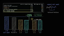
Systematic testing across six cutoff dates and seven services showed that under zero-shot conditions both versions reduced forecast error by about 25% relative to a seasonal baseline. With the holiday calendar added, both models improved further. You may not have noticed that on this dataset, version 2.5 made slightly better use of the extra inputs and produced more reliable uncertainty intervals, while 3.0's inference was several times faster.

Business Scenario Stress Test: Accurate Forecasts ≠ Correct Decisions

Continuing an existing pattern is one thing; using forecasts to make business decisions is another. The author built a multi-region software business simulation called Lumen, containing nearly four years of daily trial and revenue data, along with planned variables such as marketing spend, promotions, pricing, and holidays. Because it is a simulated environment, the true outcome of any plan is known, allowing fair scoring.

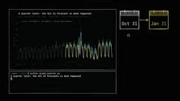
The basic forecasting capability test produced impressive results: on a database branch that excluded September and October data, TimesFM 3.0 completed a two-month forecast in under a second, with revenue deviation within 2%. The author also built a nightly pipeline in which scheduled Neon functions queue and execute tasks. When the October 31 forecast was reviewed a quarter later, 3.0's revenue deviation was still within 6%, and neither version exceeded its own uncertainty interval.

With basic accuracy established, the author handed real planning questions to a Gemini agent: the marketing team had two options—Option A deepened the Black Friday discount, while Option B kept Black Friday unchanged but doubled the January marketing budget; finance also wanted to know the impact of a January 1 price increase. Each option ran on a separate Neon branch without touching production data.

The results exposed the soft spot of zero-shot models. On the price increase question, the agent behaved correctly: after checking the historical data and finding that pricing had never changed in four years, it told finance not to trust any price-increase forecast. But on the marketing budget question, the two versions gave diametrically opposite answers—3.0 barely reacted to doubling the January budget, while 2.5 predicted a large jump in revenue. The agent chose to trust 3.0 and recommended Option A, when the true outcome was that Option B brought in more revenue. Across three rounds of testing, the agent chose wrong in two.

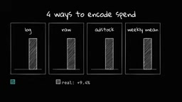
The author further ruled out numeric-format interference by testing 3.0's response under four different encodings of marketing spend, with a consistent conclusion: the model lacks reliable responsiveness to large changes beyond the historical range.

Neon is a serverless Postgres platform whose core feature is database branching: like Git branches, it can instantly create data copies from a production database for testing, simulation, or what-if analysis without touching production data at all. In this article's Lumen simulation, the author's nightly pipeline queues and executes forecasting tasks through scheduled Neon functions, and each marketing or pricing option runs on an independent branch, making it safe to compare multiple hypothetical scenarios in parallel. This "branching + scheduled functions" combination lets zero-shot forecasting models be embedded into real business processes at low cost—forecasting tasks run automatically on schedule, and results are written to isolated branches for agents or analysts to read. What needs to be distinguished is that database branching solves the problem of data isolation and orchestration; it does not improve the model's own forecasting ability. Whether the model is reliable for scenarios beyond the historical distribution still depends on the range of variation covered by the training data.

Four Limitations You Must Know Before Going to Production

First, the model can only extrapolate levers that actually moved in your history. If a variable like pricing never changed in the historical data, no zero-shot model can know your customers' price elasticity. This is not a problem unique to foundation models—traditional machine learning models are equally limited—and the solution is to run small-scale controlled experiments.

Second, beware of changes far outside the distribution. When a plan pushes budget or promotions far beyond the historical range, 2.5 and 3.0 may diverge severely. Before making decisions based on what-if forecasts, you should sanity-check against the actual lift from past campaigns rather than letting a single model version pick the winner for you.

Third, calibrate the uncertainty intervals. On the New York subway data, 3.0's confidence intervals were too narrow. Before going to production, be sure to backtest on historical data and check whether the frequency of actual values falling within the interval matches expectations.

Fourth, mind the licensing differences. Self-hosting TimesFM 3.0 falls under a non-commercial license, and commercial access must be routed through Google Cloud; 2.5, by contrast, is open source under Apache 2.0.

Conclusion: Trust It for Continuing Patterns, Not for Strategic What-Ifs

Back to the core question: is a model that has never seen your data reliable enough? For continuing existing patterns, the answer is yes—both versions beat the classic baselines zero-shot and remained within their forecast intervals a quarter later, with 3.0 holding a clear speed advantage. But for what-if planning decisions, the ceiling of a time series model is determined by the historical variation present in your data. As the video author put it, a confident forecast can cost you real money.