How Computer Simulation Designs a CT Scanner: Modeling and Simulation Methods for Five Key Components

Introduction: Why CT Design Cannot Do Without Computer Simulation

Designing a real CT scanner involves many obstacles that are difficult to overcome in practice: patients cannot be repeatedly exposed to X-ray radiation, machines cannot be arbitrarily disassembled and reassembled, and many experiments simply cannot be conducted due to ethical and cost constraints. It is precisely under these limitations that computer simulation has become an irreplaceable core tool in the CT design process.

A brilliant analogy helps illustrate this point: simulation is to CT what a wind tunnel is to aircraft. Every dangerous, non-compliant, or time-constrained experiment can first be "flown" in a computer model. The definition of computer simulation is actually quite straightforward — using theoretical models to predict real system performance. This methodology enables designers to repeatedly verify and iterate on various parameter configurations before manufacturing physical prototypes, dramatically reducing R&D costs and timelines.

The importance of computer simulation in medical device design far exceeds that of general industrial applications. CT scanners are classified as high-risk medical devices, subject to strict regulation by agencies such as the FDA (U.S. Food and Drug Administration) and NMPA (China's National Medical Products Administration). Every design change requires substantial supporting validation data. Traditional physical experimentation not only faces ethical review (human experiments involving ionizing radiation must pass IRB ethics committee approval), but a single CT prototype can cost millions of dollars to manufacture, with iteration cycles measured in months or even years. Computer simulation compresses this process to hours or days, allowing engineers to explore thousands of parameter combinations in a virtual environment, dramatically accelerating the entire journey from concept design to product finalization.

This article outlines the two major methodological frameworks for CT simulation, modeling approaches for five key components, and the engineering wisdom of cross-validating "back-of-the-envelope estimates" with full simulations throughout the process.

Two Major Simulation Methods: Analytical and Statistical

CT simulation methods fall into two main categories, each with its own applicable scenarios, advantages, and limitations.

Analytical Methods: Efficient Mathematical Modeling

Analytical methods use known analytical equations to generate system models. The most typical example is projection generation from mathematical phantoms. Phantoms are composed of basic geometric shapes such as cylinders, ellipsoids, and rods. Given the positions of the X-ray source and detector elements, the line integral of each object along the ray path can be precisely calculated, and the total projection is the weighted sum of all objects. This approach offers high computational efficiency and is particularly suitable for geometrically regular scenarios with well-defined physical processes.

Statistical Methods: Monte Carlo Simulation

Statistical methods rely on random number generators, combined with the physical properties of interactions, to simulate system behavior. The prime example is Monte Carlo simulation used to predict scatter distributions. When objects are complex and multiple scattering events occur, analytical methods become inadequate, and Monte Carlo methods must step in — photon energies are sampled from the tube spectrum, random numbers determine interaction distances, interaction types, and scattering directions, cycling millions of times until photons reach the detector, lose all energy, or escape the system.

The Monte Carlo method is named after the Monte Carlo casino in Monaco and was pioneered by von Neumann and Ulam during the 1940s Manhattan Project, originally used to simulate neutron transport in nuclear materials. In CT simulation, Monte Carlo methods require accurate modeling of three main photon-matter interactions: the photoelectric effect (photon completely absorbed by an atom, releasing a photoelectron), Compton scattering (photon undergoes inelastic scattering with an outer-shell electron, changing both energy and direction), and Rayleigh scattering (photon undergoes elastic scattering with the entire atom, changing only direction). The probability of each interaction is determined by corresponding cross-section data, typically sourced from NIST's (National Institute of Standards and Technology) XCOM database. Commonly used Monte Carlo simulation tools include GEANT4, MCNP, and EGSnrc.

From an application perspective, CT simulation primarily serves two domains: system optics concerns geometric factors — how focal spot size, detector element size, and source-to-detector and source-to-isocenter distances affect spatial resolution; system physics concerns the processes themselves — how material attenuation properties, beam hardening, and similar phenomena degrade image quality.

Modeling Five Key CT System Components

A CT system can be roughly divided into five major components: X-ray generation, scan object, photon detection and signal generation, mechanical structure, and image reconstruction. This article focuses on the first four, since the fifth — image generation — can itself be considered a form of computer simulation.

First Stop: X-ray Tube and Energy Spectrum Modeling

Photons are produced by high-speed electrons bombarding a target material, then must pass through filtration layers of oil, aluminum, copper, and other materials before reaching the patient. The energy spectrum thus profoundly influences CT image quality.

Clinical protocol selection requires careful consideration: brain examinations must distinguish gray and white matter that differ by only a few tens of HU, where low-energy photons are crucial for low-contrast resolution; while internal auditory canal examinations look at bony structures with contrast exceeding 1000 HU and are much more tolerant of noise. Through simulation, designers can precisely balance tube voltage, body-size-adaptive tube current, and filtration configurations to find optimal parameter combinations for different clinical applications.

Second Stop: Photon-Object Interactions

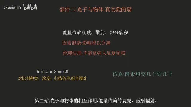
Energy-dependent attenuation, scatter radiation, partial volume effects — while these can be studied through real experiments, isolating the influence of each factor is extremely difficult. X-rays are definitively harmful, and regulations and ethics draw firm boundaries; when studying the relationship between motion and image quality, patients cannot be repeatedly exposed.

Simulation has none of these constraints — you can control exactly which factors to include and combine them however you wish, providing tremendous freedom for system physics research.

Third Stop: Detection System Modeling

Detector geometry, Detective Quantum Efficiency (DQE), and electronic noise must all be accurately predicted before physical prototypes are built. Detectors are expensive to manufacture, and iterating on geometric parameters through physical prototyping has unacceptable cycle times; lifetime specifications through accelerated aging tests are slow and confounded by factors like tube aging. Simulation enables rapid evaluation of different detector designs during the design phase.

Detective Quantum Efficiency (DQE) is a comprehensive metric measuring a detector's ability to convert incident X-ray photons into useful signals, defined as the ratio of the squared output signal-to-noise ratio to the squared input signal-to-noise ratio. A DQE of 100% means the detector perfectly preserves all statistical information in the incident radiation, while actual detectors always have DQE below 100% due to incomplete photon absorption, scintillator optical crosstalk, electronic noise, and other factors. CT detectors typically employ indirect conversion schemes (scintillators such as GOS or CsI convert X-rays to visible light, which photodiodes then convert to electrical signals) or direct conversion schemes (such as CdTe/CZT, which directly convert X-rays to electrical charge). Next-generation photon-counting detectors use direct conversion technology, offering higher DQE and energy-resolved information, and are considered a major breakthrough direction in CT detector technology.

Fourth Stop: Mechanical Structure and Alignment Tolerances

The so-called "quarter-detector offset" requires the detector's isocenter channel to be offset by exactly one-quarter of an element width — elements are approximately one millimeter wide while the source-to-detector distance is about one meter, making precise mechanical alignment practically impossible. Only simulation can determine the acceptable alignment tolerance range to ensure manufacturing precision meets imaging requirements.

Quarter-Detector Offset is an ingenious sampling strategy that improves spatial resolution without increasing the number of detector elements. In a full 360-degree scan, projection data at 0° and 180° are geometrically redundant (conjugate rays). If the detector center is precisely offset from the rotation center by one-quarter of a detector element width, then the 0° and 180° sampling points interleave by exactly half an element spacing, effectively doubling the sampling density. According to the Nyquist-Shannon sampling theorem, doubling the sampling density means the maximum resolvable spatial frequency also doubles. This technique demands extremely high mechanical precision — for a 1.0 mm element pitch, the quarter offset is only 0.25 mm, and with a source-to-detector distance of approximately one meter, angular precision must reach sub-milliradian levels. This is precisely why simulation is indispensable for tolerance analysis.

Back-of-the-Envelope Estimation: Quick Prediction of Isocenter Resolution

Before deploying full simulations, learning "back-of-the-envelope" quick estimation offers three major benefits:

1. Narrowing the parameter range, reducing the number of full simulation runs needed
2. Independent verification of simulation results — large codebases inevitably contain bugs, and obvious deviations from theoretical predictions serve as debugging clues
3. Providing quick performance insights when no simulation tools are available

Taking isocenter MTF (Modulation Transfer Function) estimation as an example, we need to introduce the concept of projected response: the response obtained by treating the focal spot as a point source and the detector element as a point is called the projected detector response; the response obtained by treating the detector element as a point source and the focal spot as having finite size is called the projected focal spot response. When these are scaled by geometric ratios and convolved, the result is the composite system response — a direct consequence of linear systems theory.

MTF (Modulation Transfer Function) is the gold standard metric for evaluating an imaging system's spatial resolution, describing the system's ability to transfer contrast information at different spatial frequencies. An MTF value of 1 indicates perfect preservation of contrast at that frequency, while 0 indicates complete loss. In CT, the resolution limit is typically specified as the spatial frequency (in line pairs per centimeter, lp/cm) at which the MTF drops to 50% or 10%. The engineering advantage of MTF lies in its decomposition of complex imaging chains into independently analyzable subsystems — focal spot MTF, detector MTF, sampling MTF, etc., multiplied together to yield the total system MTF. This is the core convenience of linear systems theory.

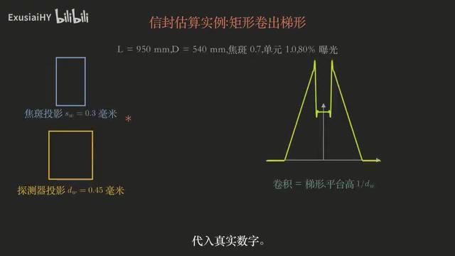
Validation with a set of real numbers: source-to-detector distance 950 mm, source-to-isocenter distance 540 mm, focal spot width 0.7 mm, element pitch 1.0 mm. Convolving two rectangles yields a trapezoidal response curve; applying a Fourier transform, multiplying by a cosine window, and taking the magnitude produces the isocenter MTF curve. When the analytical model curve and the full computer simulation curve with identical parameters are plotted together, they overlap almost perfectly — the back-of-the-envelope estimate is remarkably reliable and sufficient for quickly identifying the key factors affecting spatial resolution.

Finer Processing: Discretization Methods and Polychromatic Spectra

Handling Spatial Non-uniformity of the Focal Spot

The default assumption is that the focal spot appears as the same stationary function for all channels, but reality almost never cooperates. Due to the line-focus principle, the focal spot appears rectangular when viewed from the isocenter direction, but degrades to a T-shape when viewed off-center, with its shape noticeably deteriorating as a function of detector angle.

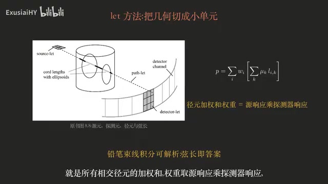
When the intensity is spatially non-uniform, analytical model complexity immediately spirals out of control. The most common alternative is to discretize the complex geometry into small elements — the focal spot is divided into M×L sub-sources, the detector into K sub-elements, and the path between each sub-source and sub-element is approximated as a zero-width "pencil beam" ray, with weighted summation approximating the true integral. This discretization method balances accuracy with computational tractability.

Polychromatic Spectra and Beam Hardening Effects

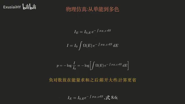
Under the monochromatic assumption, attenuation follows Beer-Lambert's Law, the fundamental physical law describing exponential attenuation of radiation in a uniform medium: I = I₀·exp(-μx), where μ is the linear attenuation coefficient and x is the penetration thickness. This law holds strictly only for monochromatic radiation. However, a real X-ray tube outputs a polychromatic spectrum — a superposition of bremsstrahlung (continuous spectrum produced by electrons decelerating in the Coulomb field of target nuclei) and characteristic radiation (line spectrum produced by inner-shell electron transitions in target atoms).

Polychromatic processing requires binning by energy, with each bin attenuating according to its own exponential law. The total transmission is the integral over all bins, and the negative logarithm operation must be applied after the energy summation — this is the mathematical root cause of beam hardening. Photons of different energies have different attenuation coefficients; low-energy photons are attenuated more strongly and are preferentially absorbed when passing through an object, causing the average energy of the transmitted beam to increase and the beam to become "harder." Mathematically, taking the negative logarithm of a polychromatic spectrum no longer yields a value linear with object thickness, causing cupping artifacts (CT values elevated at the edges and depressed at the center of a uniform water phantom) and streak artifacts (dark bands appearing between dense bones) in reconstructed images. Modern CT systems mitigate beam hardening through water correction, polynomial correction, and dual-energy imaging techniques.

Using these equations, simulation can reproduce the beam hardening artifacts in the posterior fossa — a dark band stretching between the two petrous bones, identical to typical artifacts seen in clinical CT images.

The energy spectrum also profoundly affects material contrast. Simulation experiments show that when switching to a different tube voltage, the CT value contrast between muscle and water decreases by less than 2%, while the contrast between iodinated contrast agent and water drops by nearly 18%. This is precisely because iodine's K-edge absorption makes it strongly spectrum-dependent, and contrast-enhanced examinations are highly sensitive to tube voltage.

Iodine (atomic number 53) has a K-edge energy of approximately 33.2 keV — when the X-ray photon energy just exceeds this threshold, the probability of exciting iodine's K-shell electrons surges dramatically, producing a step-function jump in the photoelectric absorption cross-section. This means photons near the K-edge are strongly absorbed by iodine, while high-energy photons far from the K-edge have greater penetrating power and reduced sensitivity to iodine. Consequently, lowering the tube voltage (e.g., from 120 kVp to 80 kVp) increases the proportion of low-energy photons near iodine's K-edge in the spectrum, significantly enhancing the CT value contrast of iodine — clinically, this is used to reduce contrast agent dose or enhance lesion visualization. Dual-Energy CT exploits differences in the attenuation characteristics of materials like iodine at different tube voltages to achieve advanced applications such as material decomposition and virtual monoenergetic imaging.

Noise Simulation and the Wisdom of Verification

Noise simulation is another important and complex area of CT simulation. Under quantum-limited conditions, CT noise modeling is more challenging than simple synthesis, with difficulties concentrated in three areas:

• Polychromatic photons follow a compound Poisson distribution, with different energy photons contributing different weights. In a polychromatic X-ray beam, the photon count in each energy bin independently follows a Poisson distribution, but since the detector responds with different weights to photons of different energies, the total signal follows a compound Poisson distribution, where the variance-to-mean relationship no longer follows the simple Poisson equality
• Preprocessing and calibration are nonlinear, meaning the processed signal no longer follows a simple Poisson distribution
• The logarithmic operation is highly nonlinear, and some calibration steps occur after the logarithmic transform

By repeatedly sampling the same path of a simulated "perfect phantom," one can clearly observe how, after all calibration steps, the signal distribution transforms from a right-skewed Poisson shape to something narrower and distorted, helping designers accurately understand how noise propagates through the entire signal processing chain.

The final lesson concerns the reliability of simulation itself: codebases are large and errors are inevitable; any simulation must be cross-checked against theoretical calculations, envelope estimates, or real experiments, and only after verification is it qualified for analyzing problems and predicting outcomes. This cross-validation mindset is the most important principle to remember in CT simulation engineering practice. In software engineering, this methodology is called "V&V" (Verification and Validation): verification answers "did we build the model correctly," and validation answers "did we build the correct model." For high-safety systems like CT, V&V is not just engineering best practice — it is a hard requirement during regulatory review.

Conclusion

Looking back at the entire methodology, CT simulation is driven by two wheels: "analytical" and "statistical." The pencil-beam ray method discretizes geometry, while Monte Carlo methods reproduce stochastic processes. This virtual CT inside the computer has become a standard tool for design specification development and reconstruction algorithm development. Once the wind tunnel is built, the next step is to send the examination table continuously through it — helical CT is about to take the stage.

Key Takeaways