Master AI Math with 5 Equations: 20 Free Python Hands-On Projects

When Machine Learning Is Distilled Down to 5 Core Equations

For many developers looking to deeply understand modern AI, the biggest barrier often isn't programming ability—it's the seemingly impenetrable mathematics. Recently, an independent machine learning engineer published a free ML workbook on Reddit with an ultra-minimalist philosophy: to understand modern AI, you only need to master 5 core equations.

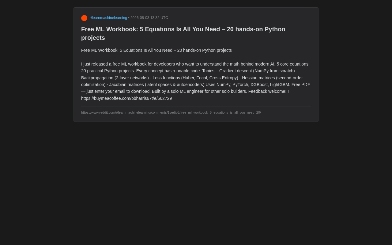
The workbook has a very clear target audience—developers who want to understand the math behind AI. Rather than piling on complex theoretical proofs, it condenses the world of machine learning into 5 key equations, accompanied by 20 runnable Python projects. Every concept has corresponding executable code, truly achieving a "learn by doing" approach.

Five Core Equations: From Beginner to Advanced

The workbook's knowledge architecture revolves around 5 mathematical tools, covering the complete path from basic optimization to advanced techniques.

Gradient Descent: The Starting Point of All Optimization

The author chose to start with Gradient Descent, emphasizing implementation from scratch using NumPy. This is a very wise pedagogical choice. Gradient descent is the foundation of virtually all deep learning optimization, and hand-coding it in pure NumPy lets learners truly understand how parameters are updated step by step, rather than treating the optimizer as a black box.

The core idea of gradient descent comes from the concept of directional derivatives in calculus. In multidimensional space, the gradient points in the direction of steepest function value increase, while the negative gradient points toward the steepest descent. The algorithm iteratively updates parameters using the formula θ = θ - α∇J(θ), where α is the learning rate and ∇J(θ) is the vector of partial derivatives of the loss function with respect to parameters. In practice, gradient descent has several variants: batch gradient descent (using all data to compute gradients), stochastic gradient descent/SGD (using only one sample at a time), and mini-batch gradient descent (a compromise between the two). Modern deep learning has also spawned adaptive learning rate optimizers like Adam and RMSProp, which essentially introduce momentum accumulation or adaptive step size adjustment mechanisms on top of basic gradient descent to handle the problem of vastly different gradient scales across parameter dimensions.

Backpropagation: The Engine of Neural Networks

The second core concept is Backpropagation, explained through a two-layer neural network. Backpropagation is the core mechanism for training neural networks, and also the part where many beginners most easily "know what but not why." Using the simplest two-layer structure as an entry point clearly demonstrates how gradients propagate layer by layer through the network.

The mathematical foundation of backpropagation is the Chain Rule from calculus. In multi-layer neural networks, computing the gradient of the output with respect to a particular layer's weights requires layer-by-layer propagation. Specifically, if a network has L layers, computing the partial derivative of the loss function with respect to layer l's weights requires multiplying all local gradients from the output layer back to layer l. This process proceeds backward from the output layer toward the input layer, hence the name "backpropagation." The 1986 paper by Rumelhart, Hinton, and Williams published in Nature formally established this algorithm's central role in neural network training. Notably, backpropagation in deep networks faces vanishing gradients (gradients decaying exponentially during propagation) and exploding gradients (gradients growing exponentially), which spurred subsequent important technical innovations like BatchNorm, residual connections (ResNet), and gating mechanisms in LSTM.

Loss Functions: The Compass for Model Learning

The workbook covers multiple Loss Functions, including Huber loss, Focal loss, and Cross-Entropy. This selection has strong practical value—cross-entropy is the standard for classification tasks, Huber loss is more robust to outliers in regression, and Focal loss is specifically designed to address class imbalance problems. This combination of three basically covers common scenarios in real-world projects.

Focal Loss was proposed by Tsung-Yi Lin et al. from Facebook AI Research (now Meta AI) in their 2017 paper "Focal Loss for Dense Object Detection," originally designed to address the severe imbalance between foreground and background samples in object detection. Its core idea is to add a modulating factor (1-p_t)^γ before the standard cross-entropy loss, where p_t is the model's predicted probability for the correct class, and γ is the focusing parameter (typically set to 2). When a sample is correctly classified with high confidence, the modulating factor approaches 0, making that sample's contribution to total loss minimal; for difficult samples where the model's predictions are inaccurate, the loss weight is fully preserved. This allows the model to automatically "focus" on hard samples during training without being dominated by large numbers of easy negative samples in gradient update direction—a design particularly useful in scenarios with extreme class imbalance such as medical image diagnosis and fraud detection.

Second-Order Optimization and Latent Spaces

The advanced section introduces the Hessian matrix (for second-order optimization) and the Jacobian matrix (for latent spaces and autoencoders). These two concepts typically appear in more advanced textbooks. The Hessian matrix describes the curvature information of the loss surface and forms the basis for second-order optimization methods like Newton's method; the Jacobian matrix is particularly important for understanding latent space transformations in Autoencoders. Combining these two more theoretical tools with practical projects is what distinguishes this workbook from ordinary beginner tutorials.

The Hessian matrix is a square matrix composed of a function's second-order partial derivatives. For a model with n parameters, it's an n×n matrix where the (i,j)-th element is the mixed partial derivative of the loss function with respect to the i-th and j-th parameters. Newton's method uses the inverse of the Hessian to determine the optimal update step size and direction, theoretically finding extrema with quadratic convergence—far faster than first-order gradient descent's linear convergence. However, computing and storing the full Hessian matrix has O(n²) space and time costs, making it nearly infeasible for deep learning models with millions or even billions of parameters. In practice, quasi-Newton methods like L-BFGS are commonly used for approximation, or only the diagonal elements of the Hessian are used to guide step size adjustment for each parameter dimension.

The Jacobian matrix describes the first-order partial derivative relationships of vector-valued functions—if a function maps m-dimensional input to n-dimensional output, the Jacobian is an n×m matrix. In the context of autoencoders, the encoder compresses high-dimensional input data (such as a 784-pixel handwritten digit image) into a low-dimensional latent space (such as 2 or 10 dimensions), and the decoder reconstructs it back to the original dimension. The Jacobian matrix characterizes the local linear approximation of this mapping—it tells us how small changes in input space affect changes in the latent representation. In models like Variational Autoencoders (VAE) and Contractive Autoencoders, analysis and regularization of the Jacobian is a core technique: contractive autoencoders penalize the Frobenius norm of the encoder's Jacobian, forcing the model to be insensitive to small input perturbations, thereby learning more robust and meaningful feature representations.

Tool Chain Covering the Mainstream Ecosystem

Notably, this workbook isn't limited to a single framework but spans multiple mainstream tools:

• NumPy: For implementing algorithms from scratch to understand the mathematical essence
• PyTorch: One of the most popular deep learning frameworks today
• XGBoost and LightGBM: Two major gradient boosting tree libraries, widely used in structured data tasks and Kaggle competitions

This tool combination reflects the author's pragmatic approach. Real-world machine learning work goes far beyond deep learning—in many tabular data scenarios, XGBoost and LightGBM are often more practical and efficient than neural networks. Including these tools in the learning path makes the workbook more aligned with real engineering practice.

XGBoost (eXtreme Gradient Boosting) and LightGBM are both ensemble learning algorithms based on Gradient Boosting Decision Trees (GBDT), but differ significantly in implementation strategies. XGBoost, proposed by Tianqi Chen in 2014, uses a level-wise tree growth strategy, examining all possible split points across all features at each split, finding the optimal split through pre-sorting or approximate histogram algorithms. LightGBM, released by Microsoft in 2017, adopts a leaf-wise growth strategy, selecting the leaf node with the highest gain for splitting each time, while introducing innovations like Gradient-based One-Side Sampling (GOSS) and Exclusive Feature Bundling (EFB). These designs make LightGBM significantly faster than XGBoost on large-scale datasets while maintaining comparable or even better accuracy on most benchmarks. In Kaggle competitions and industrial structured data tasks, these two frameworks are practically standard configuration.

"Built by a Solo Developer for Solo Builders"

The author specifically mentions in the introduction that this workbook was "built by a solo ML engineer for other solo builders." This positioning is quite interesting.

In recent years, independent developers and small teams have played an increasingly important role in the AI wave. They typically lack the resources and systematic training of large companies and need to fill knowledge gaps in the most efficient way possible. A workbook condensed to 5 equations with emphasis on runnable code perfectly matches this group's need to "get started quickly and apply immediately."

The workbook is available as a free PDF—just enter your email to download. The author is also actively soliciting feedback to continuously improve the content.

Who Is This Workbook For?

Based on publicly available information, this workbook's pedagogical approach has merit: covering the widest possible range of applications with the fewest core concepts, while adhering to the principle that "every concept has runnable code." For developers with some programming background but weak mathematical foundations, this "understanding through code" approach is often more effective than purely theoretical study.

Of course, "5 equations is all you need" is more of a marketing expression for pedagogical purposes. The complete picture of modern machine learning is far more complex than 5 equations—probability theory (Bayesian inference, maximum likelihood estimation), linear algebra (eigendecomposition, SVD), information theory (KL divergence, mutual information), and other foundations are equally indispensable. This workbook is better suited as a stepping stone for beginners and an index for practice, helping learners build intuition about core mechanisms rather than replacing systematic study.

For developers who want to get hands-on but don't know where to start, a free, focused resource with complete code like this is still worth trying.